Implementation of PCA reduction in Python

By Deepshi Sharma

In the last tutorial, I have given a brief introduction and intuition regarding Principal component analysis. If you haven’t read that post, then please go through that post before going through this post. This post will focus on implementation of PCA reduction in Python.

Link to the data set that I have used is Wine.csv

Implementation of PCA reduction :

• The first step is to import all the necessary Python libraries.

    import numpy as np
    import matplotlib.pyplot as plt
    import pandas as pd

• Import the data set after importing the libraries.

    data = pd.read_csv('Wine.csv')

• Take the complete data because the core task is only to apply PCA reduction to reduce the number of features taken.

    A = data.iloc[:, 0:13].values
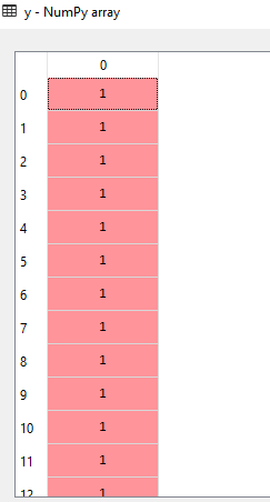
    B = data.iloc[:, 13].values

• Split the data set into training and testing data set. Below is our Python code to do this task:

    from sklearn.model_selection import train_test_split
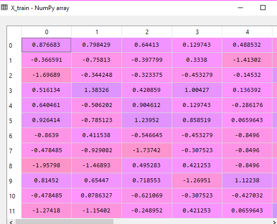
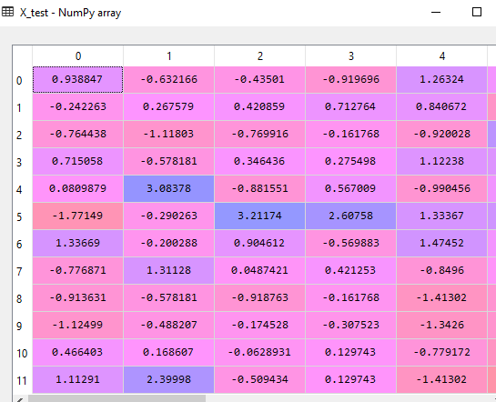
    A_train, A_test, B_train, B_test = train_test_split(A, B, test_size = 0.3)

• Now comes an important step of feature scaling so that the model is not biased towards any specific feature.

    from sklearn.preprocessing import StandardScaler
    sc = StandardScaler()
    A_train = sc.fit_transform(A_train)
    B_test = sc.transform(A_test)

• Now we will apply PCA technique. First, import PCA library and then fit the data into this. Tune the parameters as per the need of your project.

    from sklearn.decomposition import PCA
    pca = PCA(n_components = 2)
    A_train = pca.fit_transform(A_train)
    A_test = pca.transform(A_test)
    explained_variance = pca.explained_variance_ratio_

• Now when you have appropriate features. Now you can apply a suitable algorithm to get good accuracy. For example, I have used logistic regression algorithm in my model.

    from sklearn.linear_model import LogisticRegression
    classifier = LogisticRegression(random_state = 0)
    classifier.fit(A_train, B_train)

• Next step is to predict the results by using the testing set.

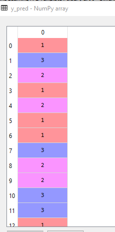
    B_pred = classifier.predict(A_test)

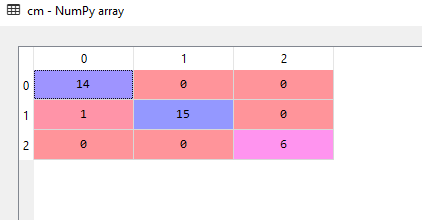
• Use any metric to evaluate your performance. For example, I have used the confusion matrix here in this program.

    from sklearn.metrics import confusion_matrix
    conf_matrix = confusion_matrix(B_test, B_pred)

Visualizing the results :

Here I will be visualizing the results that have been the outcome of the model we have created. PCA reduction has been applied.

       Visualizing training set results

    from matplotlib.colors import ListedColormap
    A_set, B_set = A_train, B_train
    X1, X2 = np.meshgrid(np.arange(start = A_set[:, 0].min() - 1, stop = A_set[:, 0].max() + 1, step = 0.01),
    np.arange(start = A_set[:, 1].min() - 1, stop = A_set[:, 1].max() + 1, step = 0.01))
    plt.contourf(A1, A2, classifier.predict(np.array([A1.ravel(), A2.ravel()]).T).reshape(A1.shape),
    alpha = 0.75, cmap = ListedColormap(('red', 'green', 'blue')))
    plt.xlim(A1.min(), A1.max())
    plt.ylim(A2.min(), A2.max())
    for i, j in enumerate(np.unique(B_set)):
    plt.scatter(A_set[y_set == j, 0], A_set[y_set == j, 1],
    c = ListedColormap(('red', 'green', 'blue'))(i), label = j)
    plt.title('Logistic Regression (Training set)')
    plt.xlabel('PC1')
    plt.ylabel('PC2')
    plt.legend()
    plt.show()

     Visualizing test set results : 

    from matplotlib.colors import ListedColormap
    A_set, B_set = A_test, B_test
    A1, A2 = np.meshgrid(np.arange(start = A_set[:, 0].min() - 1, stop = A_set[:, 0].max() + 1, step = 0.01),
    np.arange(start = A_set[:, 1].min() - 1, stop = A_set[:, 1].max() + 1, step = 0.01))
    plt.contourf(A1, X2, classifier.predict(np.array([A1.ravel(), A2.ravel()]).T).reshape(A1.shape),
    alpha = 0.75, cmap = ListedColormap(('red', 'green', 'blue')))
    plt.xlim(A1.min(), A1.max())
    plt.ylim(A2.min(), A2.max())
    for i, j in enumerate(np.unique(B_set)):
    plt.scatter(A_set[y_set == j, 0], A_set[y_set == j, 1],
    c = ListedColormap(('red', 'green', 'blue'))(i), label = j)
    plt.title('Logistic Regression (Test set)')
    plt.xlabel('PC1')
    plt.ylabel('PC2')
    plt.legend()
    plt.show()

With this, I would like to end this post here. Feel free to ask your doubts here.

Also, give a read to Random forest for regression and its implementation.