Predicting video game sales using Machine Learning in Python

Video games have become immensely popular over the past decade. The global games market in 2019 was estimated at $148.8 billion. In this article, you’ll learn how to implement a Machine Learning model that can predict the global sales of a video game depending on certain features such as its genre, critic reviews, and user reviews in Python.

Predicting video game sales using ML

As the global sales of a video game is a continuous quantity, we’ll have to implement a regression model. Regression is a form of supervised machine learning algorithm that can predict a target variable (which should be a continuous value) using a set of independent features. Some of the applications include salary forecasting, real estate predictions, etc.

Dataset

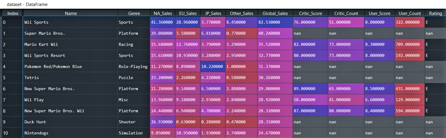
You can download the dataset from kaggle. It contains 16719 observations/rows and 16 features/columns where the features include:

NA_Sales, EU_Sales, JP_Sales: Sales in North America, Europe and Japan (in millions).
Other_Sales: Sales in other parts of the world (in millions).
Global_Sales: Total worldwide sales (in millions).
Rating: The ESRB ratings.

Code

Importing the dataset

# Importing the required libraries
import pandas as pd
import numpy as np

# Importing the dataset
dataset = pd.read_csv('Video_Games_Sales_as_at_22_Dec_2016.csv')

# Dropping certain less important features
dataset.drop(columns = ['Year_of_Release', 'Developer', 'Publisher', 'Platform'], inplace = True)

# To view the columns with missing values
print('Feature name || Total missing values')
print(dataset.isna().sum()

We drop certain features in order to reduce the time required to train the model.

OUTPUT:

Feature name || Total missing values
Name               2
Genre              2
NA_Sales           0
EU_Sales           0
JP_Sales           0
Other_Sales        0
Global_Sales       0
Critic_Score    8582
Critic_Count    8582
User_Score      9129
User_Count      9129
Rating          6769

Splitting the dataset into Train & Test sets

X = dataset.iloc[:, :].values
X = np.delete(X, 6, 1)

y = dataset.iloc[:, 6:7].values

# Splitting the dataset into Train and Test sets
from sklearn.model_selection import train_test_split
X_train, X_test, y_train, y_test = train_test_split(X, y, test_size = 0.3, random_state = 0)

# Saving name of the games in training and test set
games_in_training_set = X_train[:, 0]
games_in_test_set = X_test[:, 0]

# Dropping the column that contains the name of the games
X_train = X_train[:, 1:]
X_test = X_test[:, 1:]

Here, we initialize ‘X’ and ‘y’ where ‘X’ is the set of independent variables and ‘y’ the target variable i.e. the Global_Sales. The Global_Sales column which is present at index 6 in ‘X’ is removed using the np.delete() function before the dataset is split into training and test sets. We save the name of the games in a separate array named ‘games_in_training_set’ and ‘games_in_test_set’ as these names will not be of much help when predicting the global sales.

Imputation

Imputation in ML is a method of replacing the missing data with substituted values. Here, we’ll use the Imputer class from the scikit-learn library to impute the columns with missing values and to impute the columns with values of type string, we’ll use CategoricalImputer from sklearn_pandas and replace the missing values with ‘NA’ i.e. Not Available.

from sklearn.preprocessing import Imputer
imputer = Imputer(strategy = 'mean')
X_train[:, [5 ,6, 7, 8]] = imputer.fit_transform(X_train[:, [5, 6, 7, 8]])
X_test[:, [5 ,6, 7, 8]] = imputer.transform(X_test[:, [5, 6, 7, 8]])

from sklearn_pandas import CategoricalImputer
categorical_imputer = CategoricalImputer(strategy = 'constant', fill_value = 'NA')
X_train[:, [0, 9]] = categorical_imputer.fit_transform(X_train[:, [0, 9]])
X_test[:, [0, 9]] = categorical_imputer.transform(X_test[:, [0, 9]])

OneHotEncoding

We encode the categorical columns of ‘X’ using ColumnTransformer and OneHotEncoder from the scikit-learn library. This will assign one separate column to each category present in a categorical column of ‘X’.

from sklearn.compose import ColumnTransformer
from sklearn.preprocessing import OneHotEncoder
ct = ColumnTransformer(transformers = [('encoder', OneHotEncoder(), [0, 9])], remainder = 'passthrough') 
X_train = ct.fit_transform(X_train)
X_test = ct.transform(X_test)

Building the model

We’ll implement our model i.e. the regressor using XGBRegressor (where XGB stands for extreme gradient boosting). XGBoost is an ensemble machine learning algorithm based on decision trees similar to the RandomForest algorithm. However, unlike RandomForest that makes use of fully grown trees, XGBoost combines trees that are not too deep. Also, the number of trees combined in XGBoost is more in comparison to RandomForest. Ensemble algorithms effectively combine weak learners to produce a strong learner. XGBoost has additional features focused on performance and speed when compared to gradient boosting.

from xgboost import XGBRegressor
model = XGBRegressor(n_estimators = 200, learning_rate= 0.08)
model.fit(X_train, y_train)

Making predictions on the Test set

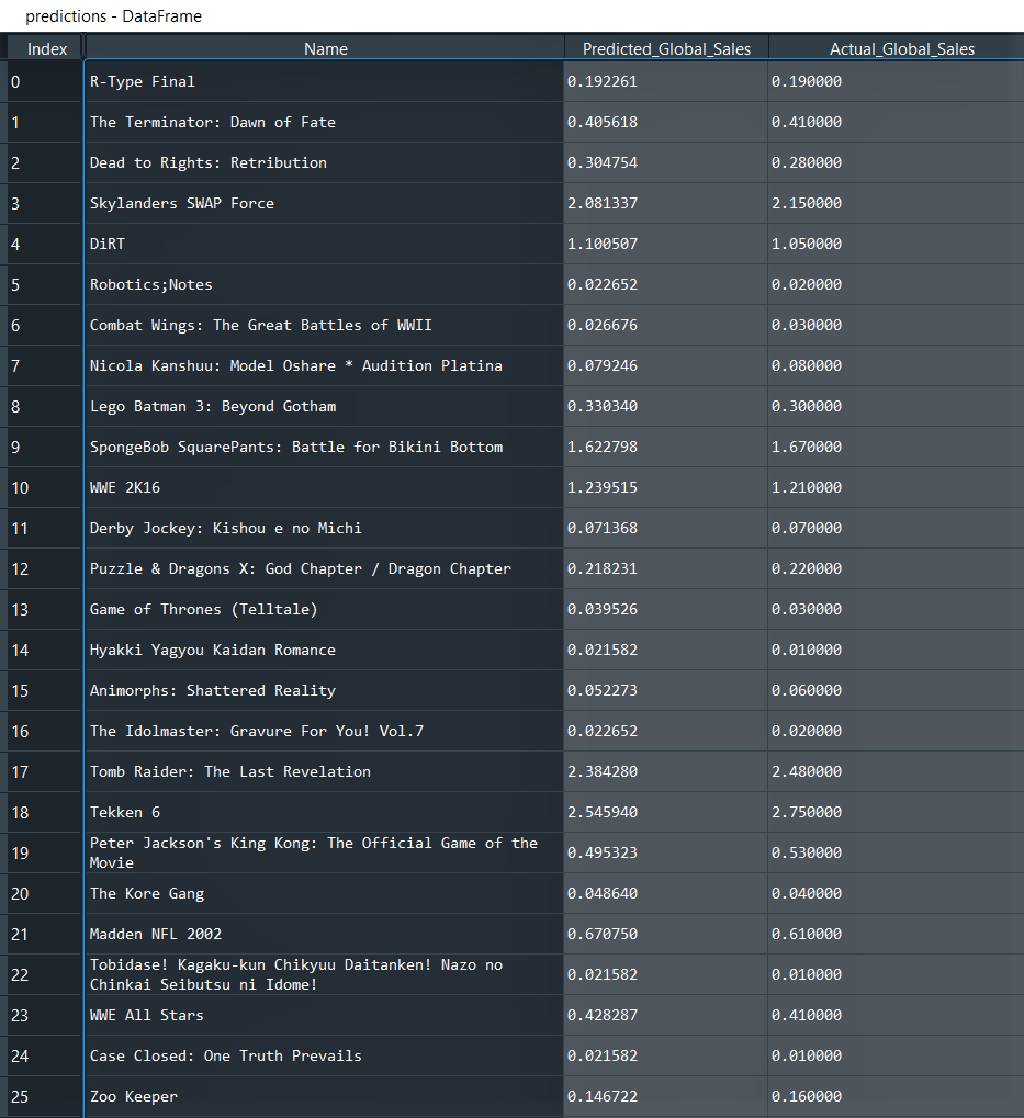
Global Sales i.e. the target variable ‘y’ for the games in the test set is predicted using the model.predict() method.

# Predicting test set results
y_pred = model.predict(X_test)

# Visualising actual and predicted sales
games_in_test_set = games_in_test_set.reshape(-1, 1)
y_pred = y_pred.reshape(-1, 1)
predictions = np.concatenate([games_in_test_set, y_pred, y_test], axis = 1)
predictions = pd.DataFrame(predictions, columns = ['Name', 'Predicted_Global_Sales', 'Actual_Global_Sales'])

First few rows of the ‘predictions’ data frame:

Evaluating model performance

We’ll use r2_score and root mean squared error (RMSE) to evaluate the model performance where closer the r2_score is to 1 & lower the magnitude of RMSE, the better the model is.

from sklearn.metrics import r2_score, mean_squared_error
import math
r2_score = r2_score(y_test, y_pred)
rmse = math.sqrt(mean_squared_error(y_test, y_pred))

print(f"r2 score of the model : {r2_score:.3f}")
print(f"Root Mean Squared Error of the model : {rmse:.3f}")