Malaria Image prediction in Python using Machine Learning
 By Anish Banerjee
In this tutorial, we will be classifying images of Malaria infected Cells. This dataset from Kaggle contains cell images of Malaria Infected cells and non-infected cells. To achieve our task, we will have to import various modules in Python. We will be using Google Colab To Code.
Modules can be directly installed through the “$ pip install” command in Colab in case they are not already present there.
We will be importing Pandas to import dataset, Matplotlib and Seaborn for visualizing the Data, sklearn for algorithms,train_test_split for splitting the dataset in testing and training set, classification report and accuracy_score for calculating accuracy of the model.
We will also be making a CNN model to do the classification test on the image dataset.
Mounting Drive
Colab being the most preferred IDE for ML projects for its powerful kernel but temporary uploaded files disappear and have to be re-uploaded after kernel session ends. So we link the drive so that it can access the dataset from there.
So it is recommended you upload the dataset in your drive.
# Run this cell to mount your Google Drive.
from google.colab import drive
drive.mount('/content/drive')
Drive already mounted at /content/drive; to attempt to forcibly remount, call drive.mount("/content/drive", force_remount=True).
Unzipping zip file from drive
We have the dataset in a zip file that we have to unzip to read or work with here.
from zipfile import ZipFile
file_name = "/content/drive/My Drive/DATASETS/cell-images-for-detecting-malaria.zip"
with ZipFile(file_name,'r') as zip:
  zip.extractall()
  print('Done')
Done.
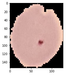
Plotting to visualize the data
import matplotlib.pyplot as plt
im = plt.imread('/content/cell_images/Parasitized/C33P1thinF_IMG_20150619_114756a_cell_180.png')
plt.imshow(im)
plt.show()
Multiple random data plot
Displaying or plotting random images to visualize them.
%matplotlib inline
import os
import matplotlib.pyplot as plt
import matplotlib.image as mpimg #The image module supports basic image loading, rescaling and display operations.

train_parasitized_fnames = os.listdir("/content/cell_images/Parasitized")
train_uninfected_fnames = os.listdir("/content/cell_images/Uninfected")
nrows = 3
ncols = 3
pic_index = 0
pic_index += 4
next_para_pix = [os.path.join("/content/cell_images/Parasitized", fname)
               for fname in train_parasitized_fnames[pic_index-4:pic_index]]
next_un_pix = [os.path.join("/content/cell_images/Uninfected", fname)
               for fname in train_uninfected_fnames[pic_index-4:pic_index]]
fig=plt.gcf()
fig.set_size_inches(ncols*4,nrows*4)
for i, img_path in enumerate(next_para_pix+next_un_pix):
  sp = plt.subplot(nrows, ncols, i + 1)
  img = mpimg.imread(img_path)
  plt.imshow(img)

plt.show()

Installing Split Folders
This will be required to split the data into train and test sets.
pip install split-folders
Collecting split-folders
  Downloading
https://files.pythonhosted.org/packages/32/d3/3714dfcf4145d5afe49101a9ed36659c3832c1e9b4d09d45e5cbb736ca3f/split_folders-0.2.3-py3-none-any.whl
Installing collected packages: split-folders
Successfully installed split-folders-0.2.3
Splitting data with a ratio of 80% and 20% for train and test sets.
The dataset needs to break into an 80% and 20% ratio to train the first part and test the trained model with the second part to check the accuracy of the model.
# Split with a ratio.
# To only split into training and validation set, set a tuple to `ratio`, i.e, `(.8, .2)`.
import split_folders
split_folders.ratio("/content/cell_images", output="output", seed=1337, ratio=(.8, .2)) # default values
Data Pre-Processing using Image Data Generator
Preprocessing the train and test data with feature changes like rescaling, rotation, width shifting, height shifting, shearing, zooming, flipping.
from tensorflow.keras.preprocessing.image import ImageDataGenerator
# All images will be rescaled by 1./255
train_data = ImageDataGenerator(
    rescale=1./255,
    rotation_range=40,
    width_shift_range=0.2,
    height_shift_range=0.2,
    shear_range=0.2,
    zoom_range=0.2,
    horizontal_flip=True,)

test_data = ImageDataGenerator(rescale=1./255)

train_generator = train_data.flow_from_directory(
        "/content/output/train",
        target_size=(150, 150),  # All images will be resized to 150x150
        batch_size=20,
        class_mode='binary')

validation_generator = test_data.flow_from_directory(
        "/content/output/val",
        target_size=(150, 150),
        batch_size=20,
        class_mode='binary')
Found 22046 images belonging to 2 classes. Found 5512 images belonging to 2 classes.
Creating a CNN Model architecture
We make a CNN architecture with convolution, pooling layers followed by activation functions. After making this repetitive structure we insert a dense layer for classification. (you can change according to your preference)
from tensorflow.keras import layers
from tensorflow.keras import Model
from tensorflow.keras.optimizers import RMSprop

img_input = layers.Input(shape=(150, 150, 3))

x = layers.Conv2D(16, 3, activation='relu')(img_input)
x = layers.MaxPooling2D(2)(x)

x = layers.Conv2D(32, 3, activation='relu')(x)
x = layers.MaxPooling2D(2)(x)

x = layers.Convolution2D(64, 3, activation='relu')(x)
x = layers.MaxPooling2D(2)(x)

x = layers.Convolution2D(128, 3, activation='relu')(x)
x = layers.MaxPooling2D(2)(x)

x = layers.Flatten()(x)

x = layers.Dense(512, activation='relu')(x)

x = layers.Dropout(0.5)(x)

output = layers.Dense(1, activation='sigmoid')(x)

model = Model(img_input, output)
Compiling the created model
from tensorflow.keras.preprocessing.image import img_to_array
from tensorflow.keras.optimizers import Adadelta

model.compile(loss='binary_crossentropy',
             optimizer=Adadelta(lr=1.0, rho=0.95, epsilon=None, decay=0.0),
             metrics=['acc'])
Checking Accuracy of the model: Malaria Image prediction in Python
After the model is ready we should train and see how the accuracy is of the trained model.
history = model.fit_generator(
     train_generator,
     steps_per_epoch=100,  # 2000 images = batch_size * steps
     epochs=15,
     validation_data=validation_generator,
     validation_steps=50,  # 1000 images = batch_size * steps
     verbose=2)
Epoch 1/15
100/100 - 17s - loss: 0.6936 - acc: 0.5285 - val_loss: 0.6569 - val_acc: 0.6040
Epoch 2/15
100/100 - 15s - loss: 0.6308 - acc: 0.6665 - val_loss: 0.4139 - val_acc: 0.8710
Epoch 3/15
100/100 - 14s - loss: 0.4123 - acc: 0.8350 - val_loss: 0.2166 - val_acc: 0.9290
Epoch 4/15
100/100 - 14s - loss: 0.2927 - acc: 0.8910 - val_loss: 0.1708 - val_acc: 0.9510
Epoch 5/15
100/100 - 14s - loss: 0.2749 - acc: 0.8985 - val_loss: 0.1786 - val_acc: 0.9590
Epoch 6/15
100/100 - 14s - loss: 0.2518 - acc: 0.9079 - val_loss: 0.1789 - val_acc: 0.9560
Epoch 7/15
100/100 - 15s - loss: 0.2658 - acc: 0.9115 - val_loss: 0.1580 - val_acc: 0.9560
Epoch 8/15
100/100 - 15s - loss: 0.2652 - acc: 0.9055 - val_loss: 0.1620 - val_acc: 0.9530
Epoch 9/15
100/100 - 14s - loss: 0.2339 - acc: 0.9180 - val_loss: 0.2087 - val_acc: 0.9570
Epoch 10/15
100/100 - 14s - loss: 0.2875 - acc: 0.9040 - val_loss: 0.1560 - val_acc: 0.9610
Epoch 11/15
100/100 - 14s - loss: 0.2432 - acc: 0.9160 - val_loss: 0.1579 - val_acc: 0.9520
Epoch 12/15
100/100 - 15s - loss: 0.2367 - acc: 0.9170 - val_loss: 0.1463 - val_acc: 0.9570
Epoch 13/15
100/100 - 14s - loss: 0.2425 - acc: 0.9175 - val_loss: 0.1532 - val_acc: 0.9590
Epoch 14/15
100/100 - 15s - loss: 0.2419 - acc: 0.9185 - val_loss: 0.1424 - val_acc: 0.9620
Epoch 15/15
100/100 - 14s - loss: 0.2569 - acc: 0.9125 - val_loss: 0.1466 - val_acc: 0.9570
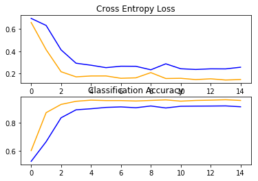
Plotting the train and test accuracy
import sys
from matplotlib import pyplot
# plot loss
pyplot.subplot(211)
pyplot.title('Cross Entropy Loss')
pyplot.plot(history.history['loss'], color='blue', label='train')
pyplot.plot(history.history['val_loss'], color='orange', label='test')
# plot accuracy
pyplot.subplot(212)
pyplot.title('Classification Accuracy')
pyplot.plot(history.history['acc'], color='blue', label='train')
pyplot.plot(history.history['val_acc'], color='orange', label='test')
pyplot.show()
Confusion Matrix
 from sklearn.metrics import confusion_matrix
from sklearn.metrics import accuracy_score
from sklearn.metrics import classification_report
results = confusion_matrix
print ('Confusion Matrix :')
print(results)
print ('Accuracy Score :',history.history['acc'] )
print ('Report : ')
print (history.history['val_acc'])
Confusion Matrix :
<function confusion_matrix at 0x7f44101d9950>
Accuracy Score : [0.503, 0.549, 0.5555, 0.6425, 0.8235, 0.87714, 0.904, 0.907, 0.9025, 0.901, 0.903, 0.9065, 0.899, 0.9135, 0.9025]
Report :
[0.51, 0.632, 0.655, 0.793, 0.866, 0.94, 0.929, 0.934, 0.942, 0.941, 0.942, 0.944, 0.949, 0.953, 0.951]
Leave a Reply