Confusion Matrix and Performance Measures in ML

Hello everyone, In this tutorial, we’ll be learning about the Confusion Matrix which is a very good way to check the performance of our Machine Learning model. We’ll see how and where it is better than the common predictive analysis tool ‘Accuracy‘ and many more. Let us start this tutorial with a brief introduction to the Confusion Matrix.

What is the Confusion Matrix and its Importance in Machine Learning

The confusion matrix is a predictive analysis tool that makes it possible to check the performance of a Classifier using various derivatives and mathematical formulae. A confusion matrix is a [2×2] matrix contains the number of true positives, true negatives, false positives, and false negatives. Using these 4 parameters we can get more precise information about the accuracy of our model.

The confusion matrix is very useful when it comes to a classification problem. What ‘Accuracy’ will tell us is the percentage of correct predictions our classifier has done out of the total. This measure is not always useful, for example, suppose we want to classify between SPAM and NOT SPAM(HAM) from a Spam detection dataset which contains 100 mails(rows) and out of that 90 are Spam and 10 are Not Spam. We build a model and what it does is predicting every mail as a Spam. So because it predicts 90 spam mails as spam we have an accuracy of 90%. But we should note that all 10 not spam(Ham) are incorrectly predicted and that’s why accuracy measure is not preferred in the Classification Tasks. To overcome the problem above we have the Confusion Matrix and its derivative measures.

Let us build a Binary Classification model using Logistic Regression and make its Confusion Matrix. This dataset is about a Product Company and includes customer details and tells whether they will buy a particular product or not.

Social_Network_Ads.csv – download the dataset.

See the code below and try to understand, we are going in deep to describe all process in this tutorial.

import pandas as pd

data = pd.read_csv(r'D:\Social_Network_Ads.csv')


x= data.iloc[:,1:-1].values
y=data.iloc[:,-1].values

from sklearn.preprocessing import LabelEncoder 
lx = LabelEncoder()
x[:,0] = lx.fit_transform(x[:,0])


##  splitting  ##
from sklearn.model_selection import train_test_split
x_train,x_test,y_train,y_test = train_test_split(x,y,test_size=0.25)

##  scaling  ##

from sklearn.preprocessing import StandardScaler
scale = StandardScaler()

x_train = scale.fit_transform(x_train)
x_test = scale.transform(x_test)


##  logistic regresion   ##

from sklearn.linear_model import LogisticRegression
logreg = LogisticRegression()
logreg.fit(x_train,y_train)

y_pred_train = logreg.predict(x_train)
y_pred_test = logreg.predict(x_test)

Confusion Matrix of above Classifier

We have successfully trained our model and now let us see the confusion matrix for our model.

from sklearn.metrics import confusion_matrix
cm = confusion_matrix(y_test,y_pred_test)

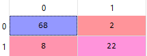
We see it is a 2 X 2 matrix with the 4 values as follows. 0 means that the Person will Not Buy a Product and 1 means that Person will Buy.

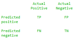
Let us see what these 4 values actually mean. Here we have taken that Buying a product is positive(1) and will make all predictions in the context of buying a product.

• True Positive – This shows the no. of items having Actual True value and classifier’s prediction is also True. Means our classifier Prediction about a positive value is Correct. In our example, If our classifier predicts that Person will Buy the Product and actually he buys it. This is True positive, something that is a predicted positive and correctly like a good bulb predicted as good.
• True Negative  – True Negative means something that is Correctly predicted and the prediction is negative. For example, If Classifier predicts that a person will not buy the product and he actually doesn’t buy it. like a defective bulb is predicted defective.
• False Positive – This shows the no. of Incorrect Predictions made and prediction is positive which means that actually the item is negative. For example, we have considered not buying a product as negative but because prediction is False or incorrect our classifier predicts that the customer will buy the product or like a defective bulb is predicted as good.
• False Negative – This can be understood as an incorrect prediction made and prediction is negative. Like the Classifier predicts that the customer will not buy the product but actually he buys it or a good bulb is predicted as a defective bulb.

A nice way to remember

Don’t get confused between all these four parameters and just care about the predictions because, in the end, we want our classifier to perform well and make more and more accurate predictions. See everything in the context of predictions and its correctness. Say False Negative, Negative means that Prediction is negative and False means incorrect means that Actual value is true. similarly, we can understand all four parameters. True prediction corresponds to binary 1 which means True and False values by default will be binary 0 that is False.

Similarly, if we consider not buying a product as a positive outcome then all four values changes.

Important note from the above classifier

The Main diagonal (T.P and T.N) is the total number of correct predictions made that is (68+22) = 90 and the other diagonal (F.P +F.N) is the Number of incorrect predictions (8+2) = 10. All of these four parameters are very useful and we’ll be discussing the derivative measures from the confusion matrix. Let us conclude the Confusion matrix we get from our example considering Buying a Product as positive (1).

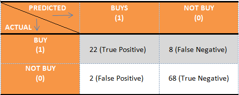
1. True Positive (T.P) = 22
2. True Negative (T.N) = 68
3. False Positive (F.P) = 2
4. False Negative (F.N) = 8

In the next section of this tutorial, we’ll be discussing the measures that we get from the Confusion.

Analytical and Performance Measures from the Confusion Matrix

Some most commonly used measures that determine the performance of a classifier derived from a confusion matrix are:

• Accuracy – Accuracy is the percentage of correct predictions that our classifier has made on the testing dataset. In confusion matrix, Correct predictions are True positive and True Negatives (T.P + T.N) while the total will be the sum of all predictions including False-positive and False-Negative(T.P + T.N + F.P + F.N). therefore accuracy will be-
  

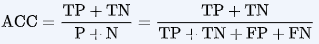
In our example, accuracy will be (22+68)/(22+68+8+2) = 0.9 or 90%

• Precision – Precision is the ratio of correct positive prediction (T.P) from the total number of positive predictions (T.P + F.P) i.e how many positive predictions made by the classifier are correct from the total. The mathematical formula for Precision is –

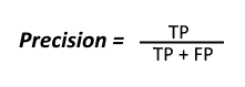
In our example, precision will be (22)/(22+2) = 0.916 or 91.6%.

• Recall – Recall is the ratio of the number of correctly predicted true value (T.P) from the total number of actual true values (T.P + F.N). In simple words, No. of correctly predicted Spams from total number of Spams. F.N means that predicted negative and false prediction means the actual value is true. The mathematical formula for Recall is-

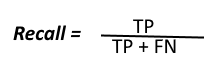
In our example, Recall will be (22)/(22+8) = 0.733 = 73.3%.

• F1_Score – F1_Score or F_measure is the harmonic mean of the Recall and Precision. In a classifier model, it is obvious that if we have a high Precision then we will get a low recall value and vice-versa. Therefore to get a measure in which both recall and precision get equal weight we make use of harmonic mean which is best for cases like these.

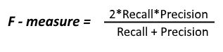
In our example, F1_Score will be (2 * 73.3 * 91.6)/(73.3 + 91.6) = 81.4%.

We hope you like this tutorial and if you have any doubts feel free to leave a comment below.

You may like to read

How to plot ROC Curve using Sklearn library in Python