COVID-19 Outbreak Prediction Using Machine Learning in Python
 By Sarbajit De
Here, we are going to discuss a burning topic COVID-19 outbreak and its prediction using various libraries in Python. This code will help us to understand the various factors of the coronavirus outbreak. After this, I am also going to provide you a dataset. Even more, I am going to evaluate those data in the dataset and predict a future model for this disease. Let’s now move forward to understand the code
Check this file below:
Python code to predict COVID-19 outbreak
import numpy as np
import pandas as pd
import matplotlib.pyplot as plt
import matplotlib.colors as mcolors
import random
import math
import time
from sklearn.model_selection import RandomizedSearchCV,train_test_split
from sklearn.svm import SVR
from sklearn.metrics import mean_squared_error, mean_absolute_error
import datetime
import operator
plt.style.use('seaborn')
confirmed_cases=pd.read_csv('Directory')
deaths_reported=pd.read_csv('Directory')
recovered_cases=pd.read_csv('Directory')
confirmed_cases.head()
deaths_reported.head()
recovered_cases.head()
cols=confirmed_cases.keys()
confirmed=confirmed_cases.loc[:, cols[4]:cols[-1]]
death=deaths_reported.loc[:, cols[4]:cols[-1]]
recoveries=recovered_cases.loc[:, cols[4]:cols[-1]]
confirmed.head()
dates=confirmed.keys()
world_caes=[]
total_deaths=[]
mortality_rate=[]
total_recovered=[]
for i in dates:
confirmed_sum=confirmed[i].sum()
death_sum=deaths[i].sum()
recovered_sum=recoveries[i].sum()
worldcases.append(confirmed_sum)
total_deaths.append(death_sum)
mortality_rate.append(death_sum/confirmed_sum)
total_recovered.append(recovered_sum)
days_since_1_22=np.array([i for i in range(len(dates))]).reshape(-1,1)
world_cases=np.array(world_cases).reshape(-1,1)
total_deaths=np.array(total_deaths).reshape(-1,1)
total_recovered=np.array(total_recovered).reshape(-1,1)
days_in_future=15
future_forcast=np.array([i for i in range(len(dates)+days_in_future)]).reshape(-1,1)
adjusted_dates=future_forcast[:10]
start='1/22/2020'
start_date=datetime.datetime.striptime(start, '%m/%d/%Y')
future_forcast_dates=[]
for i in range(len(future_forcast)):
future_forcast_dates.append(start_date+datetime.timedelta(days=i)).strftime('%m/%d/%y')
unique_countries=list(confirmed_cases['Country/Region'].uniqye())
country_confirmed_cases=[]
no_cases=[]
for i in unique_countries:
cases=latest_confirmed[confirmed_cases['Country/Region']==i].sum()
if cases>0:
country_confirmed_cases.append(cases)
else:
no_cases.append(i)
for i in no_cases:
unique_countries.remove(i)
unique_countries=[k for k,v in sorted(zip(unique_countries, country_confirmed_cases),key=operator.itemgetter(1),reverse=True)]
for i in range(len(unique_countries)):
country_confirmed_cases[i]=latest_confirmed[confirmed_caese['Country/Region']==unique_countries[i]].sum()
unique_provinces=list(confirmed_cases['Province/State'].unique())
outliers=['United Kingdom','Denmark','France']
for i in outliers:
unique_provinces.remove(i)
province_confirmed_cases=[]
no_cases=[]
for i in unique_province:
caes=latest_confirmed[confirmed_cases['Province/State']==i].sum()
if cases>0:
province_confirmed_cases.append(cases)
else:
no_cases.append(i)
for i in no_cases:
unique_province.remove(i)
for i in range(len(unique_provinces)):
print(f"{unique_provinces[i]}:{province_confirmed_cases[i]} cases")
nan_indices=[]
for i in range(len(unique_provinces)):
if type(unique_provinces[i]) == float:
nan_indices.append(i)
unique_provinces=list(unique_provinces)
provinces_confirmed_cases=list(province_confirmed_cases)
for i in nan_indices:
unique_provinces.pop(i)
provinces_confirmed_cases.pop(i)
plt.figure(figsize=(32, 32))
plt.barh(unique_countries, country_confirmed_cases)
plt.title('Number of Covid-19 Confirmed cases in countries')
plt.xlabel('Number of covid-19 Confirmed Cases')
plt.show()
kernel= ['poly', 'sigmoid', 'rbf']
c=[0.01,0.1,1,10]
gamma=[0.01,0.1,1]
epsilon=[0.01,0.1,1]
shrinking=[True,False]
svm_grid={'kernel':kernel,'C':c,'gamma':gamma,'epsilon':epsilon,'shrinking':shrinking}
svm=SVR()
svm_search=RandomisedSearch(svm,svm_grid,scoring='neg_mean_squared_error',cv=3,return_train_score=True,n_jobs=-1,n_iter=40,verbose=1)
print(svm_search.best_params)
svm_confirmed=svm_search.best_estimator_
svm_pred=svm_confirmed.predict(future_forecast)
svm_test_pred=svm_confirmed.predict(x_test_confirmed)
plt.plot(svm_test_pred)
plt.plot(y_test_confirmed)
print('MAE:',mean_absolute_error(svm_test_pred,y_test_pred))
print('MSE:',mean_squared_error(svm_test_pred,y_test_pred))
plt.figure(figsize=(20, 12))
plt.plot(adjusted_dates, world_cases)
plt.title('Number of Coronavirus Cases Over Time', size=30)
plt.xlabel('Days Since 1/22/2020', size=30)
plt.ylabel('Number of Cases', size=30)
plt.xticks(size=15)
plt.yticks(size=15)
plt.show()
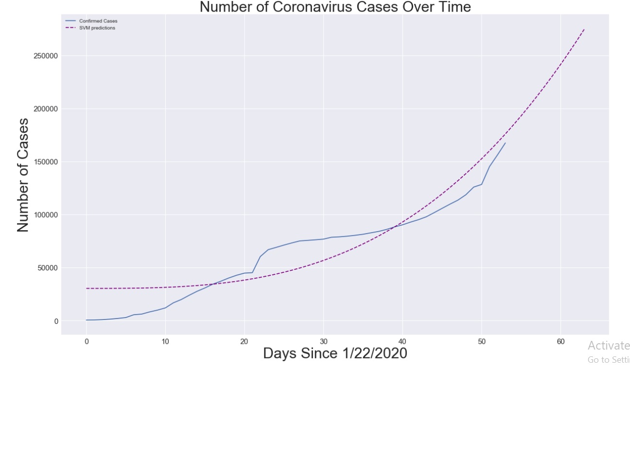
plt.figure(figsize=(20, 12))
plt.plot(adjusted_dates, world_cases)
plt.plot(future_forcast, svm_pred, linestyle='dashed', color='purple')
plt.title('Number of Coronavirus Cases Over Time', size=30)
plt.xlabel('Days Since 1/22/2020', size=30)
plt.ylabel('Number of Cases', size=30)
plt.legend(['Confirmed Cases', 'SVM predictions'])
plt.xticks(size=15)
plt.yticks(size=15)
plt.show()
from sklearn.linear_model import LinearRegression
linear_model = LinearRegression(normalize=True, fit_intercept=True)
linear_model.fit(X_train_confirmed, y_train_confirmed)
test_linear_pred = linear_model.predict(X_test_confirmed)
linear_pred = linear_model.predict(future_forcast)
print('MAE:', mean_absolute_error(test_linear_pred, y_test_confirmed))
print('MSE:',mean_squared_error(test_linear_pred, y_test_confirmed))
plt.plot(y_test_confirmed)
plt.plot(test_linear_pred)
plt.figure(figsize=(20, 12))
plt.plot(adjusted_dates, world_cases)
plt.plot(future_forcast, linear_pred, linestyle='dashed', color='orange')
plt.title('Number of Coronavirus Cases Over Time', size=30)
plt.xlabel('Days Since 1/22/2020', size=30)
plt.ylabel('Number of Cases', size=30)
plt.legend(['Confirmed Cases', 'Linear Regression Predictions'])
plt.xticks(size=15)
plt.yticks(size=15)
plt.show()
print('Linear regression future predictions:')
print(linear_pred[-10:])
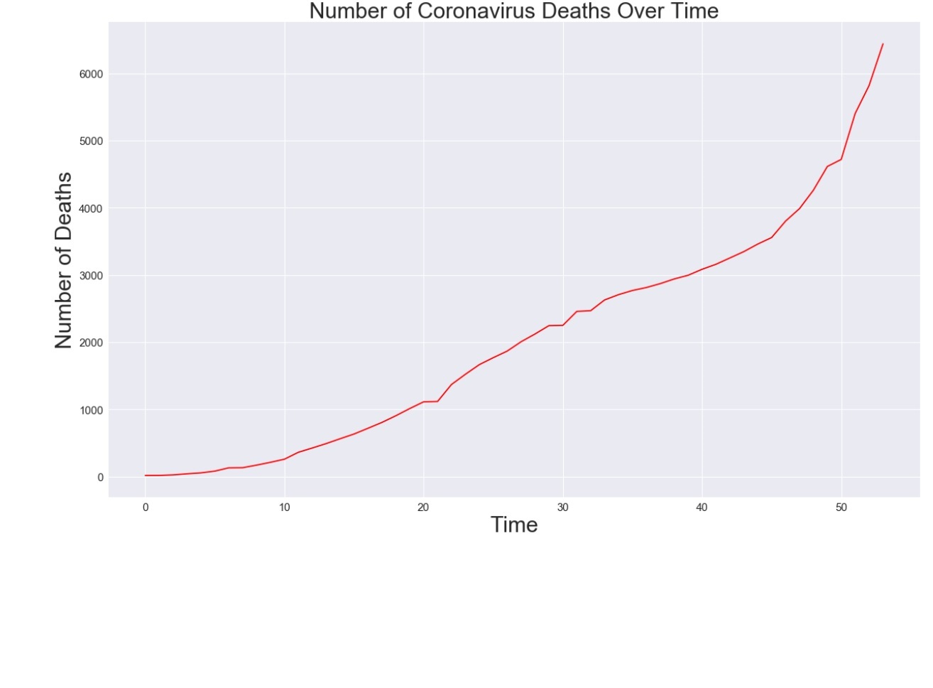
plt.figure(figsize=(20, 12))
plt.plot(adjusted_dates, total_deaths, color='red')
plt.title('Number of Coronavirus Deaths Over Time', size=30)
plt.xlabel('Time', size=30)
plt.ylabel('Number of Deaths', size=30)
plt.xticks(size=15)
plt.yticks(size=15)
plt.show()
mean_mortality_rate = np.mean(mortality_rate)
plt.figure(figsize=(20, 12))
plt.plot(adjusted_dates, mortality_rate, color='orange')
plt.axhline(y = mean_mortality_rate,linestyle='--', color='black')
plt.title('Mortality Rate of Coronavirus Over Time', size=30)
plt.legend(['mortality rate', 'y='+str(mean_mortality_rate)])
plt.xlabel('Time', size=30)
plt.ylabel('Mortality Rate', size=30)
plt.xticks(size=15)
plt.yticks(size=15)
plt.show()
plt.figure(figsize=(20, 12))
plt.plot(adjusted_dates, total_recovered, color='green')
plt.title('Number of Coronavirus Cases Recovered Over Time', size=30)
plt.xlabel('Time', size=30)
plt.ylabel('Number of Cases', size=30)
plt.xticks(size=15)
plt.yticks(size=15)
plt.show()
plt.figure(figsize=(20, 12))
plt.plot(adjusted_dates, total_deaths, color='r')
plt.plot(adjusted_dates, total_recovered, color='green')
plt.legend(['deaths', 'recoveries'], loc='best', fontsize=20)
plt.title('Number of Coronavirus Cases', size=30)
plt.xlabel('Time', size=30)
plt.ylabel('Number of Cases', size=30)
plt.xticks(size=15)
plt.yticks(size=15)
plt.show()
plt.figure(figsize=(20, 12))
plt.plot(total_recovered, total_deaths)
plt.title('Coronavirus Deaths vs Coronavirus Recoveries', size=30)
plt.xlabel('Total number of Coronavirus Recoveries', size=30)
plt.ylabel('Total number of Coronavirus Deaths', size=30)
plt.xticks(size=15)
plt.yticks(size=15)
plt.show()
Let’s Understand the working of this code:
I have a basic code where I have accepted data from datasets. Thereafter, I have arranged the data. Finally, I have tried to plot some models based on the data I have collected.
At first, I have imported all the libraries. Next, I have gathered all the data from the datasets.
Next, I have tried to predict how in future the scenarios are going to look. To do this I have used the predict function from sklearn. As a result, I have created an estimation model based on future prediction data. This is the linear regression model that I have created.
Finally, I have plotted the various data like mortality rate, death vs recovered rate, etc. This is done to visually understand the scenario.
Datasheet:
This is the datasheet I have used. To use this or some other datasheet you just change the directory. There are three datasheets and three file locations. Use them to fetch the data.
Finally, I have tried to give some visual output which I have got based on the data. I have done this with the help of the plot function. But as always predicting the future is always erroneous. It’s just a brief way to show how the expected outcome should be.
OUTPUT:


Also read: Gold Price Prediction Using Machine Learning in Python
The implementation is great but the code is incomplete hence making difficult to reproduce your results.
Copying the code directly won’t work as in machine learning you always have to make the adjustments as per your requirements. For example the file directory the path must be modified as per the path directory.
I agree with the previous comment. It is impossible to reproduce the results from your code. The main reasons are: 1) several typos in the code, and 2) python statements missing. For a person who is not familiar with the code it is difficult to guess the statements, which are important lines of the code.
The only way to help the readers is providing with the original code that you used to create the plots in the article.
Thank you
Thanks for your feedback. I will provide my code. Try to open it in jupyter notebook and copy-paste the path of your CSV file where I have placed my file directory.