How to Make Predictions with scikit-learn in Python

In this post, I’ll discuss, “How to make predictions using scikit-learn” in Python.

How to Install “scikit-learn” :

I’ll be using Python version
3.7.6 (default, Dec 19 2019, 23:50:13) \n[GCC 7.4.0]

and scikit-learn version,
sklearn.__version__
'0.22'

In Windows :
pip install scikit-learn

In Linux :
pip install --user scikit-learn

Importing scikit-learn into your Python code

import sklearn

How to predict Using scikit-learn in Python:

scikit-learn can be used in making the Machine Learning model, both for supervised and unsupervised ( and some semi-supervised problems) to predict as well as to determine the accuracy of a model!

An overview of what scikit-learn modules can be used for:

• To solve Regression problems (Linear, Logistic, multiple, polynomial regression)
• Fit and Evaluate the model
• For pre-processing a data available
• In feature extraction from categorical variables
• For Non-Linear Classification (in Decision Trees)
• In Clustering analysis

And more other advanced applications such as face-recognition, hand-writing recognition, etc…

Starting With a Simple Example:-

For Example, you have data on cake sizes and their costs :

We can easily predict the price of a “cake” given the diameter :

# program to predict the price of cake using linear regression technique
from sklearn.linear_model import LinearRegression
import numpy as np
# Step 1 : Training data
x=[[6],[8],[10],[14],[18]] # cake size (diameter) in inches
y=[[7],[9],[13],[17.5],[18]] # cake price in dollars

# step 2: Create and fit the model
model = LinearRegression()
model.fit(x,y)
size=int(input('Enter the size of the cake: '))
#step 3: make a prediction
print(f'The price of a {size}" cake would be ${model.predict(np.array([size]).reshape(1,-1))[0][0]:.02f}')

To Evaluate the model and find the fitness of the model:

To find out, that how good the prediction is,

you use the following test data set :

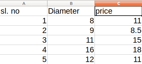
And use the following code :

## r-square using scikit learn
x_test=[8,9,11,16,12] # test
y_test=[11,8.5,15,18,11] # test
x=[[6],[8],[10],[14],[18]] # cake size (diameter) in inches
y=[[7],[9],[13],[17.5],[18]] # cake price in dollars

model= LinearRegression()
model.fit(x,y)
r_square_value=model.score(np.array(x_test).reshape(-1,1),np.array(y_test).reshape(-1,1))
print(f'r-square value from Linear Regression: {r_square_value}')

And the output is:

summary: Till now you have learned to predict the outcome of any value if it is related linearly…

Multiple Linear Regression

But suppose the cake price depends on the size of the toppings as well as the size of the cake! Then you will have to use:

And Use the following code to plot a graph against the training data set:

import matplotlib.pyplot as plt
from sklearn.linear_model import LinearRegression
x1=[[6,2],[8,1],[10,0],[14,2],[18,0]] # cake size (diameter) in inches
y=[[7],[9],[13],[17.5],[18]] # cake price in dollars
model= LinearRegression()
model.fit(x1,y)
x1_test=[[8,2],[9,0],[11,2],[16,2],[12,0]]
y_test=[[11],[8.5],[15],[18],[11]]
f=plt.figure()
ax=f.add_subplot(111)
plt.xlabel('cake size and toppings')
plt.ylabel('cake price')
predictions = model.predict(x1_test)
v1,v2=[],[]
for i,prediction in enumerate(predictions):
    print(f'predicted value : {prediction[0]:.02f} vs target value: {y_test[i][0]}')
    v1.append(prediction[0])
    v2.append(y_test[i][0])
print(f'R-squared : {model.score(x1_test,y_test)}')
ax.plot(v1,color='g',linestyle='--')
ax.plot(v2,color='r',linestyle='--')
plt.grid(True,linestyle='-',linewidth='0.5')
plt.show()
plt.close(f)

you’ll get this graph :

summary: So far you have learned about predicting data sets that are linearly related to some of the features.
Now you’ll learn how to Extract Features from Image and Pre-process data.

Extracting points of Interest from an Image and Preprocessing

Extracting Features :

# extracting points of interest from an image
# import os
import numpy as np
from skimage.feature import corner_harris,corner_peaks
from skimage.color import rgb2gray
import matplotlib.pyplot as plt
import skimage.io as io
from skimage.exposure import equalize_hist

def view_corners(corners,image):
    f = plt.figure()
    plt.gray() # converting to grayscale
    plt.imshow(image)
    y_corner , x_corner = zip(*corners)
    plt.plot(x_corner,y_corner,'x')
    plt.xlim(0, image.shape[1])
    f.set_size_inches(np.array(f.get_size_inches()) * 2.0) # to scale the display
    plt.show()
if __name__=='__main__':
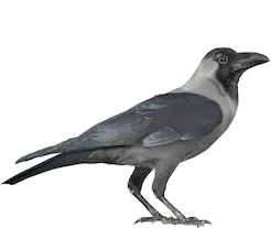
    my_image= io.imread('/home/tuhin/Pictures/crow image.jpg')
    my_image=equalize_hist(rgb2gray(my_image))
    corners = corner_peaks(corner_harris(my_image),min_distance=2)
    view_corners(corners , my_image)

image used:

the graph that you’ll see:

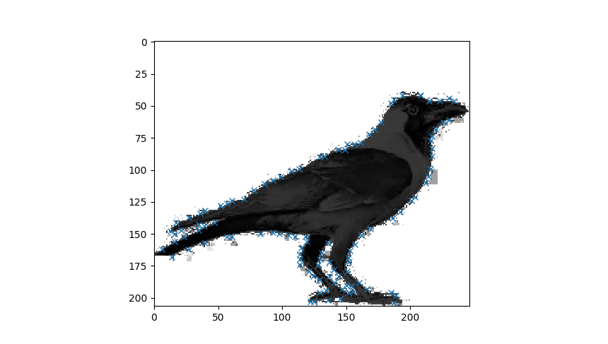
This code is capable enough of detecting the points of interest from an image,
thus it is highly relevant to use in case of HD RGB images(with lots of pixels).

Preprocessing:
Generally, predictive models perform well, when they are trained using preprocessed datasets.
# note: These types of datasets have zero mean and unit variance.

In scikit-learn, preprocessing can be done on a numpy array,
like this:

# preprocessing
from sklearn import preprocessing
import numpy as np
data = np.array([[0,1,12,4,0,0],[12,4,5,6,0,1],[0,0,0,1,1,0]])
print(preprocessing.scale(data))

Output:

[[-0.70710678 -0.39223227  1.28684238  0.16222142 -0.70710678 -0.70710678]
 [ 1.41421356  1.37281295 -0.13545709  1.13554995 -0.70710678  1.41421356]
 [-0.70710678 -0.98058068 -1.15138528 -1.29777137  1.41421356 -0.70710678]]

Logistic Regression:

This is a special case of the generalized “linear model” of scikit-learn.
This is used in classification purposes.
A very common example is “spam filtering” in messages.

Let’s take an example of the data set:

Here is a collection of some spam messages and some non-spam(ham) messages.
we’ll take the help of scikit-learn to classify spam-ham messages!

import pandas as pd
from sklearn.feature_extraction.text import TfidfVectorizer
from sklearn.linear_model.logistic import LogisticRegression
from sklearn.model_selection import train_test_split

df = pd.read_csv('/home/tuhin/Downloads/smsspamcollection/SMSSpam.csv', delimiter='\t',header=None)
print(df.head(10))
x_train_raw, x_test_raw, y_train, y_test =train_test_split(df[1],df[0]) # this function will split train and test data set in 75%-25% respectively
vector = TfidfVectorizer()
x_train = vector.fit_transform(x_train_raw)
x_test = vector.transform(x_test_raw)

classifier = LogisticRegression()
classifier.fit(x_train,y_train)
predictions = classifier.predict(x_test)

x_test_rawList = list(x_test_raw.values) # x_test_raw is in pandas dataFrame format, converting it to list
count=0
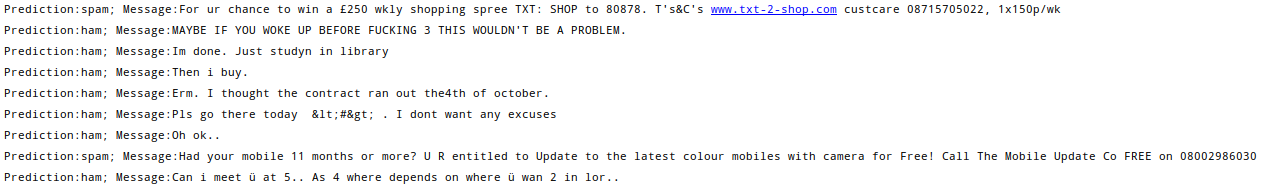
for i in predictions:
      print(f'Prediction:{i}; Message:{x_test_rawList[count]}')
      count += 1

link for the full dataset:

SMSSpam.csv

output:

And this code will predict which one is spam and which one is not!

DECISION HIERARCHY WITH scikit-learn

As in the case of non-linear regression, there are problems like decision trees
And we can also solve them using scikit-learn:

And scikit-learn’s ‘DecisionTreeClassifier’ does the job.
usage:

from sklearn.tree import DecisionTreeClassifier
from sklearn.pipeline import Pipeline
from sklearn.model_selection import GridSearchCV

pipelining = Pipeline([('clf', DecisionTreeClassifier(criterion='entropy'))])

#setting the parameters for the GridSearch
parameters = {'clf__max_depth': (150, 155, 160),'clf__min_samples_split': (1, 2, 3),'clf__min_samples_leaf': (1, 2, 3)}

# note that paramets will be different for different problems
grid_search = GridSearchCV(pipelining, parameters, n_jobs=-1,verbose=1, scoring='f1')

predictions = grid_search.predict(x_test) # we make predictions for the test data-set, where, x_test is the test_dataset

# you can get the test_data set by using train_test_split() function mentioned previously

# note: Here we count for the F1 score, of the model and that path of decision is selected, which has the best F1 score.

Clustering Methods in scikit-learn:

And there are many more clustering algorithms available under the scikit-learn module of python,
some of the popular ones are:
1. k Means clustering.

from sklearn.cluster import k_means

2. Affinity Propagation

usage: from sklearn.cluster import affinity_propagation

3. Mini Batch KMeans

usage: from sklearn.cluster import MiniBatchKMeans

4. Spectral Clustering:

usage: from sklearn.cluster import SpectralClustering

5. spectral biclustering:

usage: from sklearn.cluster import SpectralBiclustering

6. spectral-co-clustering:

usage: from sklean.cluster import SpectralCoclustering

#note: Many other clustering algorithms are available under “sklearn.cluster”.
These are some of them because it is not possible to list them in a single post!