Neural style transfer in TensorFlow – Python
 By Vanshikha Sharma
In this tutorial, we will learn about Neural style transfer in TensorFlow. In this algorithm, we optimize the loss functions to get pixel values. Neural Style transfer takes two images and merges them to get us an image that is a perfect blend. It is used in art generation where we take two images one style image and one general image. In this model, we convert the general image in the style of style image. This used transfer learning that uses a previously trained model to build on top of that. This is used when the data we have for our problem is very small. In this tutorial, we will use VGG-19 to build the model.
IMPORTING LIBRARIES
import os
import sys
import scipy.io
import scipy.misc
import matplotlib.pyplot as plt
from matplotlib.pyplot import imshow
from PIL import Image
from nst_utils import *
import numpy as np
import tensorflow as tf
import pprint
%matplotlib inline
Now in further few lines let us load this VGG-19 pre-trained weights to our model.
pp = pprint.PrettyPrinter(indent=4)
model = load_vgg_model("pretrained-model/imagenet-vgg-verydeep-19.mat")
pp.pprint(model)
Output:
{   'avgpool1': <tf.Tensor 'AvgPool:0' shape=(1, 150, 200, 64) dtype=float32>,
    'avgpool2': <tf.Tensor 'AvgPool_1:0' shape=(1, 75, 100, 128) dtype=float32>,
    'avgpool3': <tf.Tensor 'AvgPool_2:0' shape=(1, 38, 50, 256) dtype=float32>,
    'avgpool4': <tf.Tensor 'AvgPool_3:0' shape=(1, 19, 25, 512) dtype=float32>,
    'avgpool5': <tf.Tensor 'AvgPool_4:0' shape=(1, 10, 13, 512) dtype=float32>,
    'conv1_1': <tf.Tensor 'Relu:0' shape=(1, 300, 400, 64) dtype=float32>,
    'conv1_2': <tf.Tensor 'Relu_1:0' shape=(1, 300, 400, 64) dtype=float32>,
    'conv2_1': <tf.Tensor 'Relu_2:0' shape=(1, 150, 200, 128) dtype=float32>,
    'conv2_2': <tf.Tensor 'Relu_3:0' shape=(1, 150, 200, 128) dtype=float32>,
    'conv3_1': <tf.Tensor 'Relu_4:0' shape=(1, 75, 100, 256) dtype=float32>,
    'conv3_2': <tf.Tensor 'Relu_5:0' shape=(1, 75, 100, 256) dtype=float32>,
    'conv3_3': <tf.Tensor 'Relu_6:0' shape=(1, 75, 100, 256) dtype=float32>,
    'conv3_4': <tf.Tensor 'Relu_7:0' shape=(1, 75, 100, 256) dtype=float32>,
    'conv4_1': <tf.Tensor 'Relu_8:0' shape=(1, 38, 50, 512) dtype=float32>,
    'conv4_2': <tf.Tensor 'Relu_9:0' shape=(1, 38, 50, 512) dtype=float32>,
    'conv4_3': <tf.Tensor 'Relu_10:0' shape=(1, 38, 50, 512) dtype=float32>,
    'conv4_4': <tf.Tensor 'Relu_11:0' shape=(1, 38, 50, 512) dtype=float32>,
    'conv5_1': <tf.Tensor 'Relu_12:0' shape=(1, 19, 25, 512) dtype=float32>,
    'conv5_2': <tf.Tensor 'Relu_13:0' shape=(1, 19, 25, 512) dtype=float32>,
    'conv5_3': <tf.Tensor 'Relu_14:0' shape=(1, 19, 25, 512) dtype=float32>,
    'conv5_4': <tf.Tensor 'Relu_15:0' shape=(1, 19, 25, 512) dtype=float32>,
    'input': <tf.Variable 'Variable:0' shape=(1, 300, 400, 3) dtype=float32_ref>}
This gives information about the layers of the model.
In this model, We have two cost functions namely style cost function and content cost function which we will assemble together to get out the final cost function to minimize. First, let us talk about Content Cost function.
CONTENT COST FUNCTION
The image of the Louvre Museum in Paris is used as content image. This is the base image which will be styled by the end of this tutorial. So let’s import it. The generated image is going to be matching this content image.
content = scipy.misc.imread("images/louvre.jpg")
imshow(content);
Now that we have imported the image we will work on the definition of a Content cost function. A content cost function is defined as follows:
J_{content}(C,G) = *1/(4*n_H * n_W * n_C))* (a^{(C)} – a^{(G)})^2
def compute_content_cost(a_C, a_G):
    # Retrieve dimensions from a_G
    m, n_H, n_W, n_C = a_G.get_shape().as_list()

    a_C_unrolled = tf.reshape(a_C, shape=[m, n_H * n_W, n_C])
    a_G_unrolled = tf.reshape(a_G, shape=[m, n_H * n_W, n_C])

    # compute the cost with TensorFlow
    J_content = (1/(4*n_H*n_W*n_C))*tf.reduce_sum(tf.square(tf.subtract(a_C_unrolled, a_G_unrolled)))
    return J_content
tf.reset_default_graph()

with tf.Session() as test:
    tf.set_random_seed(1)
    a_C = tf.random_normal([1, 4, 4, 3], mean=1, stddev=4)
    a_G = tf.random_normal([1, 4, 4, 3], mean=1, stddev=4)
    J_content = compute_content_cost(a_C, a_G)
    print("J_content = " + str(J_content.eval()))
Output:
J_content = 6.76559
This is the value of J_contents cost function. This cost function has a hidden layer and basically tells how different the content image and generated image is. This ensures that when we minimize the cost function later G has the same content as C.
STYLE COST FUNCTION
We will import the style image that we will use here.
style_image = scipy.misc.imread("images/monet.jpg")
imshow(style_image);
Style Matrix:
- Its second name is gram matrix.
- This matrix compares the similarity between the two pictures.
In neural style transfer, the Gram matrix is computed using the following formula:
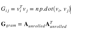
def gram_matrix(A):
    GA = tf.matmul(A,tf.transpose(A))
    return GA

tf.reset_default_graph()

with tf.Session() as test:
    tf.set_random_seed(1)
    A = tf.random_normal([3, 2*1], mean=1, stddev=4)
    GA = gram_matrix(A)

    print("GA = \n" + str(GA.eval()))
Output:
GA =
[[  6.42230511  -4.42912197  -2.09668207]
 [ -4.42912197  19.46583748  19.56387138]
 [ -2.09668207  19.56387138  20.6864624 ]]
This is the Gram Matrix. Now we will get style cost from this Gram matrix. We are using one hidden layer and the style cost function will be as follows:

G (s, gram) is Gram matrix of style image and G(G,gram) is a Gram matrix for the generated image. Let us convert this into a function.
def compute_style_cost_layer(a_S, a_G):
    # Retrieve dimensions from a_G
    m, n_H, n_W, n_C = a_G.get_shape().as_list()

    a_S = tf.transpose(tf.reshape(a_S, ([n_H*n_W, n_C])))
    a_G = tf.transpose(tf.reshape(a_G, ([n_H*n_W, n_C])))


    GS = gram_matrix(a_S)
    GG = gram_matrix(a_G)


    J_style_layer = 1./(4*n_C**2 *(n_H*n_W)**2)*tf.reduce_sum(tf.pow((GS - GG), 2))
    return J_style_layer
tf.reset_default_graph()

with tf.Session() as test:
    tf.set_random_seed(1)
    a_S = tf.random_normal([1, 4, 4, 3], mean=1, stddev=4)
    a_G = tf.random_normal([1, 4, 4, 3], mean=1, stddev=4)
    J_style_layer = compute_layer_style_cost(a_S, a_G)

    print("J_style_layer = " + str(J_style_layer.eval()))
Output:
J_style_layer = 9.19028
Till now we have taken the stye cost from only one layer. It would be more accurate if we add the cost of different layers too. We will give weights to different layers to give importance to important layers. Let’s first give the weight.
STYLE_LAYERS = [
    ('conv1_1', 0.2),
    ('conv2_1', 0.2),
    ('conv3_1', 0.2),
    ('conv4_1', 0.2),
    ('conv5_1', 0.2)]
We can combine style costs for different layers as follows:

Let’s write a function for the same.
def compute_style(model, STYLE_LAYERS):

    J_style = 0

    for layer_name, coeff in STYLE_LAYERS:


        output = model[layer_name]


        a_S = sess.run(output)


        a_G = output


        J_style_layer = compute_style_cost_layer(a_S, a_G)


        J_style += coeff * J_style_layer

    return J_style
COST OPTIMIZATION
Minimizing the total cost function step is as follows:
def total_cost(J_content, J_style, alpha = 10, beta = 40):
    J = alpha*J_content + beta*J_style
    return J
tf.reset_default_graph()

with tf.Session() as test:
    np.random.seed(3)
    J_content = np.random.randn()
    J_style = np.random.randn()
    J = total_cost(J_content, J_style)
    print(str(J))
Output:
35.34667875478276
Now we will put all the functions above together to give us the results.
tf.reset_default_graph()

sess = tf.InteractiveSession()
Working on content and style images.
content_image = scipy.misc.imread("images/louvre_small.jpg")
content_image = reshape_and_normalize_image(content_image)

style_image = scipy.misc.imread("images/monet.jpg")
style_image = reshape_and_normalize_image(style_image)
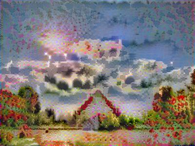
We will now create a generated image that will be co-related to content image but mostly will be a noise image.
generated_image = generate_noise_image(content_image)
imshow(generated_image[0]);

Let us call the above content cost and style functions in this running session now.
sess.run(model['input'].assign(content_image))


output = model['conv4_2']


a_C = sess.run(output)


a_G = output


J_content = compute_content_cost(a_C, a_G)


sess.run(model['input'].assign(style_image))


J_style = compute_style(model, STYLE_LAYERS)
We will work on calling the total cost function with alpha =10 and beta=40.
J = total_cost(J_content,J_style,alpha=10,beta=40)
We will be using adam optimizer with a learning rate of 0.2 for our model.
# define optimizer
optimizer = tf.train.AdamOptimizer(2.0)


train_step = optimizer.minimize(J)
Let us compile and train our model now.
def model_nn(sess, input_image, num_iterations = 200):
    sess.run(tf.global_variables_initializer())


    sess.run(model["input"].assign(input_image))


    for i in range(num_iterations):


        sess.run(train_step)


        generated_image = sess.run(model['input'])


        if i%20 == 0:
            Jt, Jc, Js = sess.run([J, J_content, J_style])
            print("Iteration " + str(i) + " :")
            print("total cost = " + str(Jt))
            print("content cost = " + str(Jc))
            print("style cost = " + str(Js))


            save_image("output/" + str(i) + ".png", generated_image)


    save_image('output/generated_image.jpg', generated_image)

    return generated_image
model_nn(sess, generated_image)
Output:
Iteration 180 :
total cost = 9.7414e+07
content cost = 18489.9
style cost = 2.43073e+06
In conclusion, We have learned about transfer learning and style and content cost functions. We can use this in many applications which is a very interesting part of this method.
Leave a Reply