Network Intrusion detection System using Machine Learning

Machine learning is one of the fastest-growing domains in technology and is finding applications in numerous fields. The ability to look for patterns in data using ML-techniques has great scope. One such use is in computer network safety. A great problem in today’s digital age is the presence of hackers, malware, and security threats on the internet. Fortunately, since internet protocols often follow fixed and predictable patterns,  Machine Learning algorithms can detect threats.

In this tutorial, we shall implement a network intrusion detection system on the famous KDD Cup 1999 Dataset in Python programming. This dataset was released as part of a data mining challenge and is openly available on UCI.

Background on data :

The extensive dataset has 495000 records, 41 input features, and 1 target variable, which tells us the status of the network activity. The network activity can be normal (no threat) or it can belong to one of the 22 categories of network attacks. To make things simpler, we will group the attacks into 4 main categories, namely :

• DOS: denial-of-service, e.g. syn flood
• R2L: unauthorized access from a remote machine, e.g. guessing password
• U2R: unauthorized access to local superuser (root) privileges, e.g., various buffer overflow attacks
• probing: surveillance and other probing, e.g., port scanning.

Initial Set up

We will first read in the data and make our observations. Below we are importing all the required Python libraries.

import pandas as pd
import numpy as np
import scipy as sp
import matplotlib.pyplot as plt
import seaborn as sns
%matplotlib inline

Now, we check read in the data, which can be accessed via a URL link.

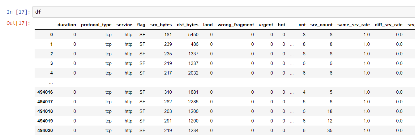
url= 'http://kdd.ics.uci.edu/databases/kddcup99/kddcup.data_10_percent.gz'
df= pd.read_csv(url, header=None)
d.head()

As you can see, there are 41 columns with the final one signifying the output to be predicted. Since the dataset doesn’t have the columns labeled beforehand, we have to do that. This information is present on the UCI dataset link.

df.columns= [ 'duration','protocol_type', 'service', 'flag', 'src_bytes','dst_bytes','land','wrong_fragment','urgent','hot','num_failed_logins','logged_in',
'num_compromised', 'root_shell', 'su_attempted', 'num_root', 'num_file_creations', 'num_shells', 'num_access_files', 'num_outbound_cmds',
'is_host_login', 'is_guest_login','cnt','srv_count','serror_rate','srv_serror_rate','rerror_rate','srv_rerror_rate','same_srv_rate',
'diff_srv_rate','srv_diff_host_rate','dst_host_count','dst_host_srv_count','dst_host_same_srv_rate','dst_host_diff_srv_rate','dst_host_same_src_port_rate',
'dst_host_srv_diff_host_rate','dst_host_serror_rate','dst_host_srv_serror_rate','dst_host_rerror_rate','dst_host_srv_rerror_rate','outcome']
print(df.describe())

Preprocessing

First, we see the target variable, outcome.

df['outcome'].unique()
>>> array(['normal.', 'buffer_overflow.', 'loadmodule.', 'perl.', 'neptune.',
       'smurf.', 'guess_passwd.', 'pod.', 'teardrop.', 'portsweep.',
       'ipsweep.', 'land.', 'ftp_write.', 'back.', 'imap.', 'satan.',
       'phf.', 'nmap.', 'multihop.', 'warezmaster.', 'warezclient.',
       'spy.', 'rootkit.'], dtype=object)

As mentioned before, we will convert it into 5 main categories, the 4 attack types listed above, and normal or safe connection.

df=df.replace(to_replace =["ipsweep.","portsweep.","nmap.","satan."],  value ="probe")
df=df.replace(to_replace =["ftp_write.", "guess_passwd.","imap.","multihop.","phf.","spy.", "warezclient.","warezmaster."],  value ="r2l")
df=df.replace(to_replace =["buffer_overflow.","loadmodule.","perl.", "rootkit."],  value ="u2r")
df=df.replace(to_replace =["back.", "land.","neptune.", "pod.","smurf.","teardrop."],value ="dos")


from collections import Counter
Counter(df['outcome'])
>>> Counter({'normal.': 97278,
         'u2r': 52,
         'dos': 391458,
         'r2l': 1126,
         'probe': 4107})

Thus, we now have only 5 output classes as listed above.

You can see that 38 attributes are numeric, while three attributes, service, protocol type, and flag contain string values that need to be converted. We do this with label encoding.

from sklearn import preprocessing 
label_encoder = preprocessing.LabelEncoder()
df['protocol_type']= label_encoder.fit_transform(df['protocol_type'])  
df['service']= label_encoder.fit_transform(df['service'])  
df['flag']= label_encoder.fit_transform(df['flag'])  
df['flag']= label_encoder.fit_transform(df['flag'])  
df['outcome']= label_encoder.fit_transform(df['outcome'])  

Since there is such a large number of features, it is possible that some features are redundant. Let us print a correlation matrix to see this.

corr = df.corr()
plt.figure(figsize=(15,12))
sns.heatmap(corr)
plt.show()

Below is the plot that we will get:

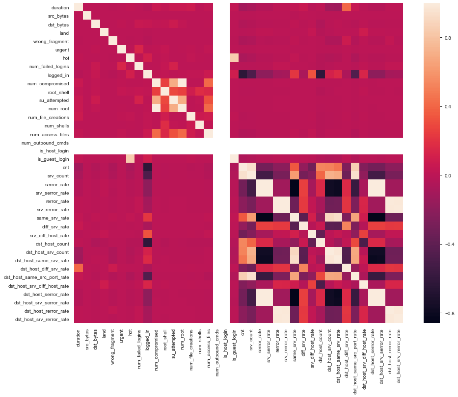
We choose columns with correlation >=0.97 as being highly correlated.

print('{:>30} {:>30} {:>30}'.format(*["Feature 1","Feature 2","Correlation"]))
x=[]
for i in c:
    for j in c:
        if((corr[i][j]>0.97) and i!=j and (i not in x)):
            l=len(i)+len(j)
            print('{:>30} {:>30} {:>30}'.format(*[i,j,corr[i][j]]))
            x.append(i)

And we will get like you can see in the image below:

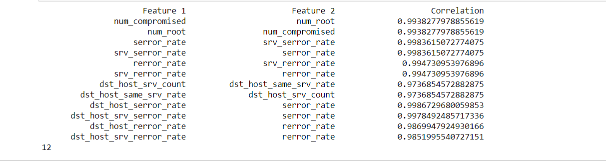
Therefore, we now drop those columns with a high correlation of 0.97 or more with other columns.

for i in x:
    if(i in df.columns):
        df.drop(i,axis=1,inplace=True)

This brings us down from 41 to 33 input features. It can be observed that two columns, ‘is_host_login’ and have all values as 0. Hence, they are redundant and can be dropped as well.

df.drop('is_host_login',axis = 1, inplace=True)
df.drop('num_outbound_cmds',axis = 1, inplace=True)

We now split it into input features and target variable, and then create the train and test dataset.

X= df.drop(['outcome'], axis=1)
Y=df['outcome']
from sklearn.model_selection import train_test_split
X_train, X_test, y_train, y_test= train_test_split(X, Y, test_size=0.2, random_state=4 )

Evaluating a model

Now, after preparing the data, it is time to select a machine learning model for it. Let us try implementing the Random-Forest classifier.

from sklearn.model_selection import train_test_split
from sklearn.metrics import confusion_matrix
from sklearn import metrics
from sklearn.ensemble import RandomForestClassifier
from sklearn.datasets import make_classification


rf = RandomForestClassifier(random_state=20,n_estimators=20)
rf.fit(X_train, y_train)

Let’s see the results of the test data.

y_preds=rf.predict(X_test)
print(confusion_matrix(y_test, y_preds))
print("Accuracy:",metrics.accuracy_score(y_test,y_preds)) 
print(metrics.classification_report(y_test,y_preds))

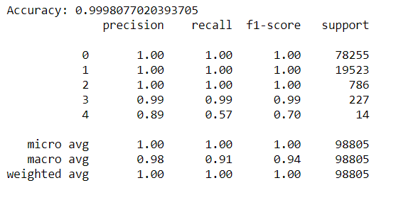
As can be seen, the model performs very well on the given dataset, with an overall accuracy of over 99%. The individual precision-recall values for the various categories are also quite high, seen from the classification report. The category ‘u2r’ doesn’t perform so well, which is due to the fact that only 52 records belong to that category.

You can try further feature selection, analysis, and use different ML algorithms.