Image to Image translation in Pytorch
 By Vikrant Dey
Image-to-image translation is a popular topic in the field of image processing and computer vision. The basic idea behind this is to map a source input image to a target output image using a set of image pairs. Some of the applications include object transfiguration, style transfer, and image in-painting.
The earliest methods used for such translations incorporated the use of Convolutional Neural Networks (CNNs). This approach minimized the loss of a pixel value between the images. But it could not produce photo-realistic images. So, recently Generative Adversarial Networks (GANs) have been of much use to the cause. Since GANs utilize adversarial feedback, the quality of image translation has improved quite a lot.
Now, this problem of image translation comes with various constraints as data can be paired as well as unpaired. Paired data have training examples with one to one correspondence, while unpaired data have no such mapping. In this tutorial, we shall see how we can create models for both paired and unpaired data. We shall use a Pix2Pix GAN for paired data and then a CycleGAN for unpaired data.
Now enough of theories; let us jump into the coding part. First, we shall discuss how to create a Pix2Pix GAN model and then a CycleGAN model.
Pix2Pix for Paired Data
The GAN architecture consists of a generator and a discriminator. The generator outputs new synthetic images while the discriminator differentiates between the real and fake (generated) images. So, this betters the quality of the images. The Pix2Pix model discussed here is a type of conditional GAN (also known as cGAN). The output image is generated conditioned on the input image. The discriminator is fed both the input and output images. Then it has to decide if the target is a variated and transformed version of the source. Then, ‘Adversarial losses’ train the generator and the ‘L1 losses’ between the generated and target images update the generator.
Applications of Pix2Pix GAN include conversion of satellite images to maps, black and white photographs to colored ones, sketches to real photos, and so on. In this tutorial, we shall discuss how to convert sketches of shoes to actual photos of shoes.
We are going to use the edges2shoes dataset which can be downloaded from the link: https://people.eecs.berkeley.edu/~tinghuiz/projects/pix2pix/datasets/edges2shoes.tar.gz
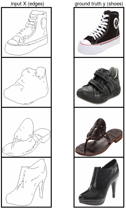
This dataset contains train and test sets of pairs of two figures in each. One is the edged outline of a shoe and the other is the original image of the shoe. Our task is to create a Pix2Pix GAN model from the data so that we can translate the outlines into real pictures of the shoes.
First, we download the dataset. Then we should separate the train and test folders from being in the same folder directory to different folders. For saving the log, we can create a separate folder, though this is optional. After that, we dive into the code.
Importing necessary libraries and modules
import os
import numpy as np
import matplotlib.pyplot as plt
import matplotlib.animation as animation
import random
import math
import io

from PIL import Image
from copy import deepcopy
from IPython.display import HTML

import torch
import torchvision
import torchvision.transforms as transforms
import torchvision.utils as vutils
import torch.nn as nn
import torch.nn.functional as F
import torch.optim as optim


device = torch.device("cuda" if torch.cuda.is_available() else "cpu")
manual_seed = ...
random.seed(manual_seed)
torch.manual_seed(manual_seed)
For working with the train and test data, we need to create data loaders. Also, we enter the necessary transformations and data inputs.
log_path = os.path.join("...") #Enter the log saving directory here

data_path_Train = os.path.dirname('...') #Enter the train folder directory
data_path_Test = os.path.dirname('...') #Enter the test folder directory

batch_size = 4
num_workers = 2

transform = transforms.Compose([transforms.Resize((256,512)),
                                transforms.ToTensor(),
                                transforms.Normalize((0.5,),(0.5,)),])

load_Train = torch.utils.data.DataLoader(torchvision.datasets.ImageFolder(root=
             data_path_Train, transform=transform), batch_size=batch_size,
             shuffle=True, num_workers=num_workers)

load_Test = torch.utils.data.DataLoader(torchvision.datasets.ImageFolder(root=
            data_path_Test, transform=transform), batch_size=batch_size,
            shuffle = False, num_workers=num_workers)
Now we shall try to view how the images in the batches look like. We have to iterate the objects in the train data loader for viewing one at a time. Then for creating the batches, we have to split the data loader.
def show_E2S(batch1, batch2, title1, title2):
    # edges
    plt.figure(figsize=(15,15))
    plt.subplot(1,2,1)
    plt.axis("off")
    plt.title(title1)
    plt.imshow(np.transpose(vutils.make_grid(batch1, nrow=1, padding=5,
    normalize=True).cpu(),(1,2,0)))
    # shoes
    plt.subplot(1,2,2)
    plt.axis("off")
    plt.title(title2)
    plt.imshow(np.transpose(vutils.make_grid(batch2, nrow=1, padding=5,
    normalize=True).cpu(),(1,2,0)))

def split(img):
    return img[:,:,:,:256], img[:,:,:,256:]

r_train, _ = next(iter(load_Train)
X, y = split(r_train.to(device), 256)
show_E2S(X,y,"input X (edges)","ground truth y (shoes)")
Output:
Building blocks of architecture
Here comes the main functional part of the code. Convolutional blocks, together with transposed convolutional blocks for upsampling, are defined here. In the later sections, we have to use these extensively.
inst_norm = True if batch_size==1 else False  # instance normalization


def conv(in_channels, out_channels, kernel_size, stride=1, padding=0):
    return nn.Conv2d(in_channels, out_channels, kernel_size, stride=stride,
    padding=padding)


def conv_n(in_channels, out_channels, kernel_size, stride=1, padding=0, inst_norm=False):
    if inst_norm == True:
        return nn.Sequential(nn.Conv2d(in_channels, out_channels, kernel_size,
        stride=stride, padding=padding), nn.InstanceNorm2d(out_channels,
        momentum=0.1, eps=1e-5),)
    else:
        return nn.Sequential(nn.Conv2d(in_channels, out_channels, kernel_size,
        stride=stride, padding=padding), nn.BatchNorm2d(out_channels,
        momentum=0.1, eps=1e-5),)

def tconv(in_channels, out_channels, kernel_size, stride=1, padding=0, output_padding=0,):
    return nn.ConvTranspose2d(in_channels, out_channels, kernel_size, stride=stride,
    padding=padding, output_padding=output_padding)

def tconv_n(in_channels, out_channels, kernel_size, stride=1, padding=0, output_padding=0, inst_norm=False):
    if inst_norm == True:
        return nn.Sequential(nn.ConvTranspose2d(in_channels, out_channels, kernel_size,
        stride=stride, padding=padding, output_padding=output_padding),
        nn.InstanceNorm2d(out_channels, momentum=0.1, eps=1e-5),)
    else:
        return nn.Sequential(nn.ConvTranspose2d(in_channels, out_channels, kernel_size,
        stride=stride, padding=padding, output_padding=output_padding),
        nn.BatchNorm2d(out_channels, momentum=0.1, eps=1e-5),)
The generator model here is basically a U-Net model. It is an encoder-decoder model with skip connections between encoder and decoder layers having same-sized feature maps. For the encoder, we have first the Conv layer, then the Batch_norm layer, and then the Leaky ReLU layer. For the decoder, we have first the Transposed Conv layer, then the Batchnorm layer, and then the (Dropout) and ReLU layers. To merge the layers with skip connections, we use the torch.cat() function.
dim_c = 3
dim_g = 64

# Generator
class Gen(nn.Module):
    def __init__(self, inst_norm=False):
        super(Gen,self).__init__()
        self.n1 = conv(dim_c, dim_g, 4, 2, 1)
        self.n2 = conv_n(dim_g, dim_g*2, 4, 2, 1, inst_norm=inst_norm)
        self.n3 = conv_n(dim_g*2, dim_g*4, 4, 2, 1, inst_norm=inst_norm)
        self.n4 = conv_n(dim_g*4, dim_g*8, 4, 2, 1, inst_norm=inst_norm)
        self.n5 = conv_n(dim_g*8, dim_g*8, 4, 2, 1, inst_norm=inst_norm)
        self.n6 = conv_n(dim_g*8, dim_g*8, 4, 2, 1, inst_norm=inst_norm)
        self.n7 = conv_n(dim_g*8, dim_g*8, 4, 2, 1, inst_norm=inst_norm)
        self.n8 = conv(dim_g*8, dim_g*8, 4, 2, 1)

        self.m1 = tconv_n(dim_g*8, dim_g*8, 4, 2, 1, inst_norm=inst_norm)
        self.m2 = tconv_n(dim_g*8*2, dim_g*8, 4, 2, 1, inst_norm=inst_norm)
        self.m3 = tconv_n(dim_g*8*2, dim_g*8, 4, 2, 1, inst_norm=inst_norm)
        self.m4 = tconv_n(dim_g*8*2, dim_g*8, 4, 2, 1, inst_norm=inst_norm)
        self.m5 = tconv_n(dim_g*8*2, dim_g*4, 4, 2, 1, inst_norm=inst_norm)
        self.m6 = tconv_n(dim_g*4*2, dim_g*2, 4, 2, 1, inst_norm=inst_norm)
        self.m7 = tconv_n(dim_g*2*2, dim_g*1, 4, 2, 1, inst_norm=inst_norm)
        self.m8 = tconv(dim_g*1*2, dim_c, 4, 2, 1)
        self.tanh = nn.Tanh()

    def forward(self,x):
        n1 = self.n1(x)
        n2 = self.n2(F.leaky_relu(n1, 0.2))
        n3 = self.n3(F.leaky_relu(n2, 0.2))
        n4 = self.n4(F.leaky_relu(n3, 0.2))
        n5 = self.n5(F.leaky_relu(n4, 0.2))
        n6 = self.n6(F.leaky_relu(n5, 0.2))
        n7 = self.n7(F.leaky_relu(n6, 0.2))
        n8 = self.n8(F.leaky_relu(n7, 0.2))
        m1 = torch.cat([F.dropout(self.m1(F.relu(n8)), 0.5, training=True), n7], 1)
        m2 = torch.cat([F.dropout(self.m2(F.relu(m1)), 0.5, training=True), n6], 1)
        m3 = torch.cat([F.dropout(self.m3(F.relu(m2)), 0.5, training=True), n5], 1)
        m4 = torch.cat([self.m4(F.relu(m3)), n4], 1)
        m5 = torch.cat([self.m5(F.relu(m4)), n3], 1)
        m6 = torch.cat([self.m6(F.relu(m5)), n2], 1)
        m7 = torch.cat([self.m7(F.relu(m6)), n1], 1)
        m8 = self.m8(F.relu(m7))

        return self.tanh(m8)
The discriminator used here is a PatchGAN model. It chops the image into overlapping pixel images or patches. The discriminator works on each patch and averages the result. Then we create a function for initialization of weights.
dim_d = 64

# Discriminator
class Disc(nn.Module):
    def __init__(self, inst_norm=False):
        super(Disc,self).__init__()
        self.c1 = conv(dim_c*2, dim_d, 4, 2, 1)
        self.c2 = conv_n(dim_d, dim_d*2, 4, 2, 1, inst_norm=inst_norm)
        self.c3 = conv_n(dim_d*2, dim_d*4, 4, 2, 1, inst_norm=inst_norm)
        self.c4 = conv_n(dim_d*4, dim_d*8, 4, 1, 1, inst_norm=inst_norm)
        self.c5 = conv(dim_d*8, 1, 4, 1, 1)
        self.sigmoid = nn.Sigmoid()

    def forward(self, x, y):
        xy=torch.cat([x,y],dim=1)
        xy=F.leaky_relu(self.c1(xy), 0.2)
        xy=F.leaky_relu(self.c2(xy), 0.2)
        xy=F.leaky_relu(self.c3(xy), 0.2)
        xy=F.leaky_relu(self.c4(xy), 0.2)
        xy=self.c5(xy)

        return self.sigmoid(xy)

def weights_init(z):
    cls_name =z.__class__.__name__
    if cls_name.find('Conv')!=-1 or cls_name.find('Linear')!=-1:
        nn.init.normal_(z.weight.data, 0.0, 0.02)
        nn.init.constant_(z.bias.data, 0)
    elif cls_name.find('BatchNorm')!=-1:
        nn.init.normal_(z.weight.data, 1.0, 0.02)
        nn.init.constant_(z.bias.data, 0)
The model is a binary classification model since it predicts only two results: real or fake. So we use BCE loss. We also need to calculate L1 losses to find the deviation between the expected and translated images. Then we use Adam optimizer for both the generator and discriminator.
BCE = nn.BCELoss() #binary cross-entropy
L1 = nn.L1Loss()

#instance normalization
Gen = Gen(inst_norm).to(device)
Disc = Disc(inst_norm).to(device)

#optimizers
Gen_optim = optim.Adam(Gen.parameters(), lr=2e-4, betas=(0.5, 0.999))
Disc_optim = optim.Adam(Disc.parameters(), lr=2e-4, betas=(0.5, 0.999))
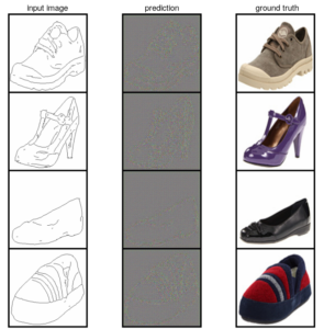
Now we shall view one instance of the input and target images along with the predicted image before training our model.
fix_con, _ = next(iter(load_Test)
fix_con = fix_con.to(device)
fix_X, fix_y = split(fix_con)


def compare_batches(batch1, batch2, title1, title2, batch3=None, title3):
    # batch1
    plt.figure(figsize=(15,15))
    plt.subplot(1,3,1)
    plt.axis("off")
    plt.title(title1)
    plt.imshow(np.transpose(vutils.make_grid(batch1, nrow=1, padding=5,
    normalize=True).cpu(), (1,2,0)))
    # batch2
    plt.subplot(1,3,2)
    plt.axis("off")
    plt.title(title2)
    plt.imshow(np.transpose(vutils.make_grid(batch2, nrow=1, padding=5,
    normalize=True).cpu(), (1,2,0)))
    # third batch
    if batch3 is not None:
        plt.subplot(1,3,3)
        plt.axis("off")
        plt.title(title3)
        plt.imshow(np.transpose(vutils.make_grid(batch3, nrow=1, padding=5,
        normalize=True).cpu(), (1,2,0)))

with torch.no_grad():
    fk = Gen(fix_X)
compare_batches(fix_X, fk, "input image", "prediction", fix_y, "ground truth")
Output:
Training the model
After the generator generates an output, the discriminator first works on the input image and the generated image. Then it works on the input image and the output image. After that, we calculate the generator and the discriminator losses. The L1 loss is a regularizing term and a hyperparameter known as ‘lambda’ weighs it. Then we add the looses together.
loss = adversarial_loss + lambda * L1_loss
img_list = []
Disc_losses = Gen_losses = Gen_GAN_losses = Gen_L1_losses = []


iter_per_plot = 500
epochs = 5
L1_lambda = 100.0


for ep in range(epochs):
    for i, (data, _) in enumerate(load_Train):
        size = data.shape[0]

        x, y = split(data.to(device), 256)

        r_masks = torch.ones(size,1,30,30).to(device)
        f_masks = torch.zeros(size,1,30,30).to(device)

        # disc
        Disc.zero_grad()
        #real_patch
        r_patch=Disc(y,x)
        r_gan_loss=BCE(r_patch,r_masks)

        fake=Gen(x)
        #fake_patch
        f_patch = Disc(fake.detach(),x)
        f_gan_loss=BCE(f_patch,f_masks)

        Disc_loss = r_gan_loss + f_gan_loss
        Disc_loss.backward()
        Disc_optim.step()

        # gen
        Gen.zero_grad()
        f_patch = Disc(fake,x)
        f_gan_loss=BCE(f_patch,r_masks)

        L1_loss = L1(fake,y)
        Gen_loss = f_gan_loss + L1_lambda*L1_loss
        Gen_loss.backward()

        Gen_optim.step()

        if (i+1)%iter_per_plot == 0 :

            print('Epoch [{}/{}], Step [{}/{}], disc_loss: {:.4f}, gen_loss: {:.4f},Disc(real): {:.2f}, Disc(fake):{:.2f}, gen_loss_gan:{:.4f}, gen_loss_L1:{:.4f}'.format(ep, epochs, i+1, len(load_Train), Disc_loss.item(), Gen_loss.item(), r_patch.mean(), f_patch.mean(), f_gan_loss.item(), L1_loss.item()))

            Gen_losses.append(Gen_loss.item())
            Disc_losses.append(Disc_loss.item())
            Gen_GAN_losses.append(f_gan_loss.item())
            Gen_L1_losses.append(L1_loss.item())

            with torch.no_grad():
                Gen.eval()
                fake = Gen(fix_X).detach().cpu()
                Gen.train()
            figs=plt.figure(figsize=(10,10))

            plt.subplot(1,3,1)
            plt.axis("off")
            plt.title("input image")
            plt.imshow(np.transpose(vutils.make_grid(fix_X, nrow=1, padding=5,
            normalize=True).cpu(), (1,2,0)))

            plt.subplot(1,3,2)
            plt.axis("off")
            plt.title("generated image")
            plt.imshow(np.transpose(vutils.make_grid(fake, nrow=1, padding=5,
            normalize=True).cpu(), (1,2,0)))

            plt.subplot(1,3,3)
            plt.axis("off")
            plt.title("ground truth")
            plt.imshow(np.transpose(vutils.make_grid(fix_y, nrow=1, padding=5,
            normalize=True).cpu(), (1,2,0)))

            plt.savefig(os.path.join(log_PATH,modelName+"-"+str(ep) +".png"))
            plt.close()
            img_list.append(figs)
An image list ‘img_list’ is created. So, if you want to create a GIF to illustrate the training procedure, you can do it by making use of the list. Moving on to the last section, we shall now view our predictions.
t_batch, _ =  next(iter(load_Test))
t_x, t_y = batch_data_split(t_batch, 256)

with torch.no_grad():
    Gen.eval()
    fk_batch=G(t_x.to(device))
compare_batches(t_x, fk_batch, "input images", "predicted images", t_y, "ground truth")
Output:
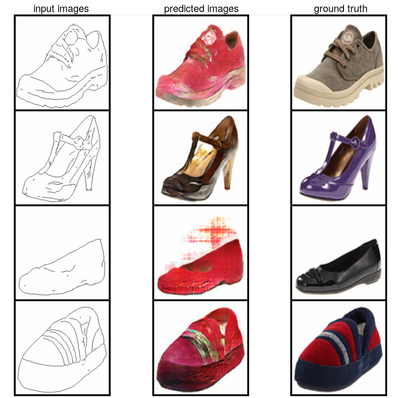
The number of epochs used here is only 5. Hence the predictions are a lot less realistic than expected. If you increase the number of epochs to 30 or more, the results will be astonishing. But it takes a lot of time to accomplish that.
The losses for this training are illustrated here:
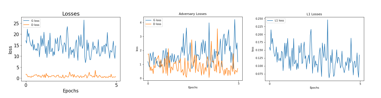
You can easily create the plots from the expressions given above. But, if you face any difficulty in plotting the data, you should look up this tutorial: https://www.codespeedy.com/plotting-mathematical-expression-using-matplotlib-in-python/
So this was the first section of this tutorial. Now we move on to working with unpaired data.
CycleGAN for Unpaired Data
CycleGAN is a recent extension of the GAN architecture. It includes parallel training of two generators and two discriminators. One generator takes images of a domain X as input and then generates fake images that look like domain Y. The other generator takes images of domain Y as input and then creates counterfeit images that look like domain X. After that, discriminators are used for determining the realism of generated images, thereby lightly improving their quality. So this is sufficient to generate plausible images of each domain.
The idea can get quite blurry. Therefore, let us illustrate this with the help of an example. Suppose, there are two generators G1 and G2, and two discriminators DX and DY being trained here. Then:
- Generator G1 learns to transform image X to image Y.
- Generator G2 learns to transform image Y to image X.
- Discriminator DX learns to differentiate between image X and generated image X.
- Discriminator DY learns to differentiate between image Y and generated image Y.
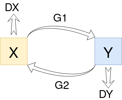
After that, a notion of cycle consistency follows. So, the cycle consistency loss compares the images and penalizes the discriminators accordingly. Soon, the regularization of CycleGAN is complete, and we have our translations ready.
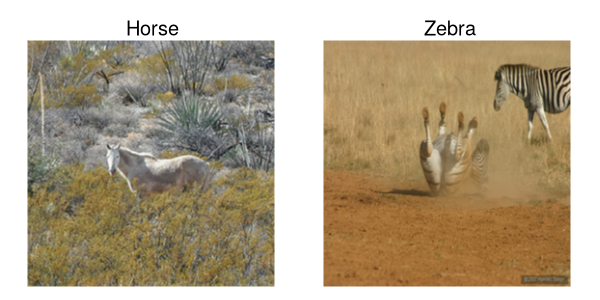
Too many theories can get boring, so let us dive into the coding section. Here, we shall work on the horse2zebra dataset which can be downloaded from the link: https://people.eecs.berkeley.edu/~taesung_park/CycleGAN/datasets/horse2zebra.zip
This dataset contains two train sets and two test sets. One train set and one test set contain images of horses, while the other train and test sets contain images of zebras. Our task is to create a CycleGAN model from the data so that we can translate from horse to zebra and then to a horse, plus zebra to a horse and then to zebra.
First, we download the dataset. Then we should separate each of the train and test folders from being in the same folder directory to four different empty folders. For saving the log, we can create a separate folder, although this is optional.
Many of the things would be a repetition from the previous section. So we shall traverse fast through here.
Importing necessary libraries + modules and building data-loaders
import os
import numpy as np
import matplotlib.pyplot as plt
import random
import math
import pickle
import torch
import torchvision
import torchvision.transforms as transforms
import torchvision.utils as vutils
import torch.nn as nn
import torch.nn.functional as F
import torch.optim as optim

device = torch.device("cuda" if torch.cuda.is_available() else "cpu")
manual_seed = ...
random.seed(manual_seed)
torch.manual_seed(manual_seed)


log_path = os.path.join("...") #optional

#data paths
data_path_Train_A = os.path.dirname('...')
data_path_Train_B = os.path.dirname('...')
data_path_Test_A = os.path.dirname('...')
data_path_Test_B = os.path.dirname('...')

batch_size = 1
inst_norm = True if batch_size==1 else False  # instance norm
num_workers = 2

transform = transforms.Compose([transforms.Resize((256,256)),
                                transforms.ToTensor(),
                                transforms.Normalize((0.5,),(0.5,)),])


# horse
load_Train_A = torch.utils.data.DataLoader(torchvision.datasets.ImageFolder(root=
               data_path_Train_A, transform=transform), batch_size=batch_size,
               shuffle =True, num_workers=num_workers)

#zebra
load_Train_B = torch.utils.data.DataLoader(torchvision.datasets.ImageFolder(root=
               data_path_Train_B, transform=transform), batch_size=batch_size,
               shuffle =True, num_workers=num_workers)

#horse
load_Test_A = torch.utils.data.DataLoader(torchvision.datasets.ImageFolder(root=
              data_path_Test_A, transform=transform), batch_size=batch_size,
              shuffle = False, num_workers=num_workers)

#zebra
load_Test_B = torch.utils.data.DataLoader(torchvision.datasets.ImageFolder(root=
              data_path_Test_B, transform=transform), batch_size=batch_size,
              shuffle = False, num_workers=num_workers)
We shall view how our domains look like.
horse_batch, _ = next(iter(load_Train_A))
zebra_batch, _ = next(iter(load_Train_B))


def show_hz(batch1, batch2, title1, title2):
    # Horse
    plt.figure(figsize=(15,15))
    plt.subplot(1,2,1)
    plt.axis("off")
    plt.title(title1)
    plt.imshow(np.transpose(vutils.make_grid(batch1, nrow=1, padding=2,
    normalize=True).cpu(), (1,2,0)))
    # Zebra
    plt.subplot(1,2,2)
    plt.axis("off")
    plt.title(title2)
    plt.imshow(np.transpose(vutils.make_grid(batch2, nrow=1, padding=2,
    normalize=True).cpu(), (1,2,0)))


show_hz(horse_batch, zebra_batch, "Horse", "Zebra")
Output:
Building blocks of architecture
So here we come to the functional part of the code. Now, we shall create functions for convolutional and transposed convolutional blocks. Then we build a Resnet block, which would be further used in building the generator function.
def conv_n(in_channels, out_channels, kernel_size, stride=1, padding=0, inst_norm=False):
    if inst_norm == True:
        return nn.Sequential(nn.Conv2d(in_channels, out_channels, kernel_size,
        stride=stride, padding=padding), nn.InstanceNorm2d(out_channels,
        momentum=0.1, eps=1e-5),)
    else:
        return nn.Sequential(nn.Conv2d(in_channels, out_channels, kernel_size,
        stride=stride, padding=padding), nn.BatchNorm2d(out_channels,
        momentum=0.1, eps=1e-5),)

def tconv_n(in_channels, out_channels, kernel_size, stride=1, padding=0, output_padding=0, inst_norm=False):
    if inst_norm == True:
        return nn.Sequential(nn.ConvTranspose2d(in_channels, out_channels,
        kernel_size, stride=stride, padding=padding, output_padding=output_padding),
        nn.InstanceNorm2d(out_channels, momentum=0.1, eps=1e-5),)
    else:
        return nn.Sequential(nn.ConvTranspose2d(in_channels, out_channels,
        kernel_size, stride=stride, padding=padding, output_padding=output_padding),
        nn.BatchNorm2d(out_channels, momentum=0.1, eps=1e-5),)


class Res_Block(nn.Module):
    def __init__(self, dim, inst_norm, dropout):
        super(Res_Block, self).__init__()
        self.cb = self.build_cb(dim, inst_norm, dropout)

    def build_cb(self, dim, inst_norm, dropout):
        cb = []
        cb += [nn.ReflectionPad2d(1)]
        cb += [conv_n(dim, dim, 3, 1, 0, inst_norm=inst_norm), nn.ReLU(True)]
        if dropout:
            cb += [nn.Dropout(0.5)]
        cb += [nn.ReflectionPad2d(1)]
        cb += [conv_n(dim, dim, 3, 1, 0, inst_norm=inst_norm)]
        return nn.Sequential(*cb)

    # skip connections
    def forward(self, x):
        out = x + self.cb(x)
        return out
Hence this having done, we have to build the generator and discriminator blocks and define the weights-initialization function. The underlying architecture is quite similar to that of a Pix2Pix GAN model. So, the generator we are using here is a U-Net model. Then you can notice that the discriminator is a PatchGAN model too.
dim_c = 3

# Number of filters in first layer of gen is nG_filter
class Gen(nn.Module):
    def __init__(self, input_nc, output_nc, nG_filter=64, inst_norm=False, dropout=False,
    num_blocks=9):
        super(Gen, self).__init__()

        mod = [nn.ReflectionPad2d(3), conv_n(dim_c, nG_filter, 7, 1, 0,
               inst_norm=inst_norm), nn.ReLU(True)]

        # downsampling
        num_down = 2
        for i in range(num_down):
            mlt = 2**i
            mod += [conv_n(nG_filter*mlt, nG_filter*mlt*2, 3, 2, 1,
                    inst_norm=inst_norm), nn.ReLU(True)]

        mlt = 2**num_down
        for i in range(num_blocks):
            mod += [Res_Block(nG_filter*mlt, inst_norm=inst_norm, dropout=dropout)]

        # upsampling
        for i in range(num_down):
            mlt = 2**(num_down - i)
            mod += [tconv_n(nG_filter*mlt, int(nG_filter*mlt/2), 3, 2, 1,
                    output_padding=1,inst_norm=inst_norm), nn.ReLU(True)]
        mod += [nn.ReflectionPad2d(3)]
        mod += [nn.Conv2d(nG_filter, output_nc, 7, 1, 0)]
        mod += [nn.Tanh()]
        self.mod = nn.Sequential(*mod)

    def forward(self, input):
        return self.mod(input)


dim_d = 64

class Disc(nn.Module):
    def __init__(self, inst_norm=False):
        super(Disc,self).__init__()
        self.c1 = conv(dim_c, dim_d, 4, 2, 1)
        self.c2 = conv_n(dim_d, dim_d*2, 4, 2, 1, inst_norm=inst_norm)
        self.c3 = conv_n(dim_d*2, dim_d*4, 4, 2, 1, inst_norm=inst_norm)
        self.c4 = conv_n(dim_d*4, dim_d*8, 4, 1, 1, inst_norm=inst_norm)
        self.c5 = conv(dim_d*8, 1, 4, 1, 1)

        self.sigmoid = nn.Sigmoid()


    def forward(self, x):
        x=F.leaky_relu(self.c1(x), 0.2)
        x=F.leaky_relu(self.c2(x), 0.2)
        x=F.leaky_relu(self.c3(x), 0.2)
        x=F.leaky_relu(self.c4(x), 0.2)
        x=self.c5(x)

        return self.sigmoid(x)

def weights(z):
    cls_name = z.__class__.__name__
    if cls_name.find('Conv')!=-1 or cls_name.find('Linear')!=-1:
        nn.init.normal_(z.weight.data, 0.0, 0.02)
        nn.init.constant_(z.bias.data, 0)
    elif cls_name.find('BatchNorm')!=-1:
        nn.init.normal_(z.weight.data, 1.0, 0.02)
        nn.init.constant_(z.bias.data, 0)
We have to define how to calculate the adversarial losses (mean squared error) and the identity losses (L1 or mean average error). After that, we need to show the calculations for the forward and backward cycle losses. Then, for the optimizers, we need to keep on feeding them the gradient of the updated weights.
MSE = nn.MSELoss()
L1 = nn.L1Loss()


Gen_A = Gen_B = Gen(dim_c, dim_c, inst_norm=inst_norm).to(device)
Disc_A = Disc_B =  Disc(inst_norm).to(device)

Gen_A_optimizer = Gen_B_optimizer = optim.Adam(Gen_A.parameters(), lr=1e-4, betas=(0.5, 0.99))
Disc_A_optimizer = Disc_B_optimizer = optim.Adam(Disc_A.parameters(), lr=1e-4, betas=(0.5, 0.99))
Before we start the training, we should look at some instances of cycles that need to be trained.
# to show 4 outputs at a time for A and B sets

A_cond = B_cond = None

for i, (t, _) in enumerate(load_Test_A):
    if i == 0:
        A_cond = t
    elif i == 4:
        break
    else:
        A_cond = torch.cat((A_cond, t), 0)

for i, (t, _) in enumerate(load_Test_B):
    if i == 0:
        B_cond = t
    elif i == 4:
        break
    else:
        B_cond=torch.cat((B_cond, t), 0)

A_cond = A_cond.to(device)
B_cond = B_cond.to(device)


def compare_batches(batch1, batch2, title1, title2, third_batch=None, title3):
    # batch1
    plt.figure(figsize=(15,15))
    plt.subplot(1,3,1)
    plt.axis("off")
    plt.title(title1)
    plt.imshow(np.transpose(vutils.make_grid(batch1, nrow=1, padding=2,
    normalize=True).cpu(), (1,2,0)))
    # batch2
    plt.subplot(1,3,2)
    plt.axis("off")
    plt.title(title2)
    plt.imshow(np.transpose(vutils.make_grid(batch2, nrow=1, padding=2,
    normalize=True).cpu(), (1,2,0)))
    # batch3
    if batch3 is not None:
        plt.subplot(1,3,3)
        plt.axis("off")
        plt.title(title3)
        plt.imshow(np.transpose(vutils.make_grid(batch3, nrow=1, padding=2,
        normalize=True).cpu(), (1,2,0)))
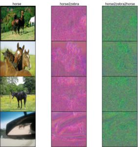
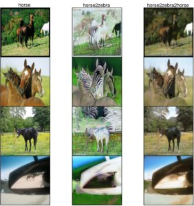
To view horse -> zebra -> horse cycle instance, we have:
with torch.no_grad():
    gen_batch = Gen_A(A_cond)
    gen_rec_batch = Gen_B(gen_batch)
compare_batches(A_cond, gen_batch, "horse", "horse2zebra", gen_rec_batch, "horse2zebra2horse")
Output:
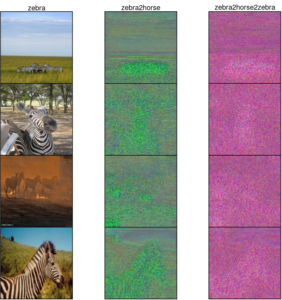
To view zebra -> horse -> zebra cycle instance, we have:
with torch.no_grad():
    gen_batch = Gen_B(B_cond)
    gen_rec_batch = Gen_A(gen_batch)
compare_batches(B_cond, gen_batch,"zebra", "zebra2horse", gen_rec_batch, "zebra2horse2zebra")
Output:
Training the model
Finally, we come to the training part. Just like the previous section, we shall create image lists too. So, if you want to create a GIF to get an idea of the training procedure, you should make use of the lists. Here, we shall calculate the losses and train our model. Most of the tasks would be just the same as in the previous section.
img_a_list = img_b_list = []

Disc_A_GAN_losses = Disc_B_GAN_losses = Gen_A_GAN_losses = Gen_B_GAN_losses = []

cycle_A_B_A_losses = cycle_B_A_B_losses = []


iter_per_plot = 250
epochs = 15

for ep in range(epochs):
    for ((i, (A_data, _)), (B_data, _)) in zip(enumerate(load_Train_A), load_Train_B):

        b_size= A_data.shape[0]

        A_data=A_data.to(device)
        B_data=B_data.to(device)

        r_mask = torch.ones(b_size,1,30,30).to(device)
        f_mask = torch.zeros(b_size,1,30,30).to(device)

        # Train Disc
        Disc_A.zero_grad()
        r_patch=Disc_A(A_data)
        r_gan_loss=MSE(r_patch,r_mask)

        fake_A = Gen_B(B_data)
        f_patch = Disc_A(fake_A.detach())
        f_gan_loss=MSE(f_patch,f_mask)

        Disc_A_GAN_loss = r_gan_loss + f_gan_loss
        Disc_A_GAN_loss.backward()
        Disc_A_optim.step()

        Disc_B.zero_grad()
        r_patch=Disc_B(B_data)
        r_gan_loss=MSE(r_patch,r_mask)

        fake_B = Gen_A(A_data)
        f_patch = Disc_B(fake_B.detach())
        f_gan_loss=MSE(f_patch,f_mask)

        Disc_B_GAN_loss = r_gan_loss + f_gan_loss
        Disc_B_GAN_loss.backward()
        Disc_B_optim.step()


        # Train Gen
        Gen_A.zero_grad()
        f_patch = Disc_B(fake_B)
        Gen_A_GAN_loss=MSE(f_patch,r_mask)

        Gen_B.zero_grad()
        f_patch = Disc_A(fake_A)
        Gen_B_GAN_loss=MSE(f_patch,r_mask)


        # h2z2h
        fake_B_A=Gen_B(fake_B)
        cycle_A_loss=L1(fake_B_A,A_data)

        # z2h2z
        fake_A_B=Gen_A(fake_A)
        cycle_B_loss=L1(fake_A_B,B_data)


        G_loss=Gen_A_GAN_loss+Gen_B_GAN_loss+ 10.0*cycle_A_loss + 10.0*cycle_B_loss
        G_loss.backward()
        Gen_A_optim.step()
        Gen_B_optim.step()

        if (i+1)%iter_per_plot == 0 :
            print('Epoch [{}/{}], Step [{}/{}], Disc_A_loss: {:.4f}, Disc_B_loss: {:.4f},Gen_A_loss: {:.4f}, Gen_B_loss:{:.4f}, A_cycle_loss:{:.4f}, B_cycle_loss:{:.4f}'.format(ep, epochs, i+1, len(load_Train_A), Disc_A_GAN_loss.item(), Disc_B_GAN_loss.item(), Gen_A_GAN_loss.item(), Gen_B_GAN_loss.item(), cycle_A_loss.item(), cycle_B_loss.item()))

            Disc_A_GAN_losses.append(Disc_A_GAN_loss.item())
            Disc_B_GAN_losses.append(Disc_B_GAN_loss.item())
            Gen_A_GAN_losses.append(Gen_A_GAN_loss.item())
            Gen_B_GAN_losses.append(Gen_B_GAN_loss.item())

            cycle_A_B_A_losses.append(cycle_A_loss.item())
            cycle_B_A_B_losses.append(cycle_B_loss.item())

            with torch.no_grad():
                Gen_A.eval()
                Gen_B.eval()
                fake_B = Gen_A(A_cond).detach()
                fake_B_A = Gen_B(fake_B).detach()
                fake_A = Gen_B(B_cond).detach()
                fake_A_B = Gen_A(fake_A).detach()
                Gen_A.train()
                Gen_B.train()

            figs=plt.figure(figsize=(10,10))
            plt.subplot(1,3,1)
            plt.axis("off")
            plt.title("horse")
            plt.imshow(np.transpose(vutils.make_grid(A_cond, nrow=1, padding=5,
            normalize=True).cpu(), (1,2,0)))
            plt.subplot(1,3,2)
            plt.axis("off")
            plt.title("horse2zebra")
            plt.imshow(np.transpose(vutils.make_grid(fake_B, nrow=1, padding=5,
            normalize=True).cpu(), (1,2,0)))
            plt.subplot(1,3,3)
            plt.axis("off")
            plt.title("horse2zebra2horse")
            plt.imshow(np.transpose(vutils.make_grid(fake_B_A, nrow=1, padding=5,
            normalize=True).cpu(), (1,2,0)))
            plt.savefig(os.path.join(log_path,modelName+"A-"+str(ep) + ".png"))
            plt.close()
            img_a_list.append(figs)

            figs=plt.figure(figsize=(10,10))
            plt.subplot(1,3,1)
            plt.axis("off")
            plt.title("zebra")
            plt.imshow(np.transpose(vutils.make_grid(B_cond, nrow=1, padding=5,
            normalize=True).cpu(), (1,2,0)))
            plt.subplot(1,3,2)
            plt.axis("off")
            plt.title("zebra2horse")
            plt.imshow(np.transpose(vutils.make_grid(fake_A, nrow=1, padding=5,
            normalize=True).cpu(), (1,2,0)))
            plt.subplot(1,3,3)
            plt.axis("off")
            plt.title("zebra2horse2zebra")
            plt.imshow(np.transpose(vutils.make_grid(fake_A_B, nrow=1, padding=5,
            normalize=True).cpu(), (1,2,0)))
            plt.savefig(os.path.join(log_path,modelName+"B-"+str(ep) +".png"))
            plt.close()
            img_b_list.append(figs)
This the last part of the code. We shall look at the outputs generated.
with torch.no_grad():
    gen_batch=Gen_A(A_cond)
    gen_rec_batch=Gen_B(gen_batch)
compare_batches(A_cond, gen_batch, "horse", "horse2zebra", gen_rec_batch, "horse2zebra2horse")
Output:
with torch.no_grad():
    gen_batch=Gen_B(B_cond)
    gen_rec_batch = Gen_A(gen_batch)
compare_batches(B_cond, gen_batch, "zebra", "zebra2horse", gen_rec_batch, "zebra2horse2zebra")
Output:
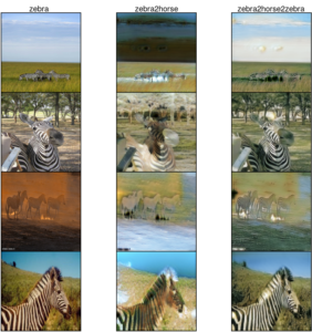
The predicted images are not realistic. This is because of the number of epochs being too low. The optimal number of epochs for this code would be >100. But, even then, good quality images can hardly be generated. Moreover, it would take a lot of time and resources to train the model. Nevertheless, this being a tutorial, it aims to illustrate an easy-to-grasp method of building models for image-to-image translation.
Hi,
could you please provide the code for plotting generator loss and discriminator loss