Decision Tree Regression in Python using scikit learn

In this tutorial, we are are going to evaluate the performance of a data set through Decision Tree Regression in Python using scikit-learn machine learning library.

What is Decision tree?

• A supervised learning method represented in the form of a graph where all possible solutions to a problem are checked.
• Decisions are based on some conditions.
• It is represented in the form of an acyclic graph.
• It can be used for both classification and regression.

Nodes in a Decision Tree

• Root Node: A base node of the entire tree.
• Parent/Child Node: Root node is considered as a parent node while all other nodes derived from root node are child nodes.
• Leaf Node: The last node that cannot be further segregated.

How does Decision tree work?

• It breaks down a dataset into smaller subsets while at the same time an associated decision tree is incrementally developed.
• In each branching node of the graph, a specified feature is being examined. If the value of the feature is below a specific threshold, the left branch is followed; otherwise, the right branch is followed.

Illustration of a decision tree.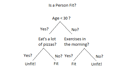 

Methods used to Evaluate Performance in Decision Tree Regression

1. Mean Absolute Error:

   Syntax:  >>from sklearn.metrics import mean_absolute_error
            >> y_true = [3,0,5]
            >> mean_absolute_error(y_true, y_predict)
   

    

2. Mean Squared Error:

   Syntax:      >>from sklearn.metrics import mean_squared_error 
                >>mean_squared_error(y_test, y_predict)

    

3. R² Score:

Syntax: >>from sklearn.metrics import r2_score 
        >> mean_absolute_error(y_true, y_predict)

Example of Decision Tree in Python – Scikit-learn

Click here to download  Melbourne Housing market dataset.

 

Importing required libraries to read our dataset and for further analyzing.

import pandas as pd
import sklearn
from sklearn import tree
from sklearn.tree import DecisionTreeRegressor

Reading.CSV file with pandas dataframe and looking its labelled columns.

melbourne_df = pd.read_csv("Melbourne_housing_FULL.csv")
melbourne_df.columns

Output:

Index(['Suburb', 'Address', 'Rooms', 'Type', 'Price', 'Method', 'SellerG',
       'Date', 'Distance', 'Postcode', 'Bedroom2', 'Bathroom', 'Car',
       'Landsize', 'BuildingArea', 'YearBuilt', 'CouncilArea', 'Lattitude',
       'Longtitude', 'Regionname', 'Propertycount'],
      dtype='object')

#The melbourne data has some missing values.
#we will learn to handle mssing values
melbourne_df.describe()

Output: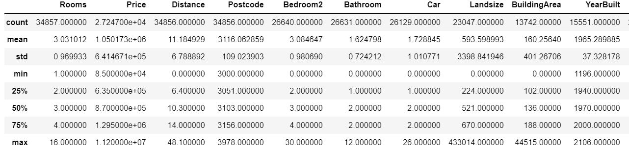 

We can see that columns such as ‘Rooms’ ‘Latitude’, ‘Longitude’ have missing values.

#We use fillna() function in order to complete missing values, with mean() values of respective columns. 

melbourne_df['Longtitude'] = melbourne_df['Longtitude'].fillna((melbourne_df['Longtitude'].mean()))
melbourne_df['Lattitude'] = melbourne_df['Lattitude'].fillna((melbourne_df['Lattitude'].mean()))
melbourne_df['Bathroom'] = melbourne_df['Bathroom'].fillna((melbourne_df['Bathroom'].mean()))
melbourne_df['Landsize'] = melbourne_df['Landsize'].fillna((melbourne_df['Landsize'].mean()))

Now we call our target value for which prediction is to be made.

y = melbourne_df.Price

#The columns that out inputted into our model are known as 'features.
#These columns are used to determine the home price.

#For now, we will build our model for only a few features.

melbourne_features = ['Rooms', 'Bathroom', 'Landsize', 'Lattitude', 'Longtitude']

X = melbourne_df[melbourne_features]

# Defining. model.
melbourne_model = DecisionTreeRegressor(random_state=42)

# Fit the model
melbourne_model.fit(X, y)

Output : DecisionTreeRegressor(criterion='mse', max_depth=None, max_features=None,
                      max_leaf_nodes=None, min_impurity_decrease=0.0,
                      min_impurity_split=None, min_samples_leaf=1,
                      min_samples_split=2, min_weight_fraction_leaf=0.0,
                      presort=False, random_state=1, splitter='best')

#We make predictions of Price for first 5 houses using Decision Tree regressor

print("The predictions for following following 5 houses:")
print(X.head())
print("The predictions made for houses are : ")
print(melbourne_model.predict(X.head()))

Output:
Predicting prices for the following 5 houses:
   Rooms  Bathroom  Landsize  Lattitude  Longtitude
0      2       1.0     126.0   -37.8014    144.9958
1      2       1.0     202.0   -37.7996    144.9984
2      2       1.0     156.0   -37.8079    144.9934
3      3       2.0       0.0   -37.8114    145.0116
4      3       2.0     134.0   -37.8093    144.9944
The predictions for prices of houses are
[1050173.34495541 1480000.         1035000.         1050173.34495541
 1465000.        ]

Also read,

• Anomaly Detection in Python using scikit learn
• Isolation Forest in Python using scikit learn