From dividing line to Support Vector Machines in Python
 By Premkumar Vemula
A simple dividing line is used to make predictions on simple 2D data where we have a dependent variable and an independent variable.
A line can be drawn according to the relation between those and following the trend of the line we can make predictions.
For example-
Here we have taken an independent dummy variable X and a dependent variable Y that takes the squared values of X.
import matplotlib.pyplot as plt
X=[1,3,5,7,8]
Y=[1,9,25,49,64]
plt.scatter(X,Y)
plt.plot(X,Y)
plt.show
Now plotting this we get a
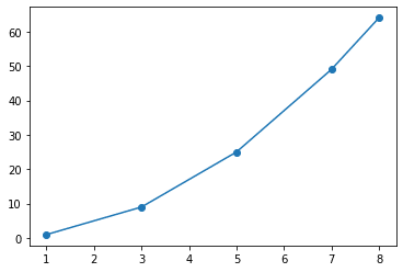
This is obviously a brute-force method. Also, most data that we encounter in our daily lives are not simple numerical values and are multidimensional.
So we need a better method to make predictions. Some of them are linear regression and logistic regression.
These algorithms learn a function and using that function it will make predictions, also called hypothesis.
Linear regression assumes a linear relationship between the dependent and the independent variable, while logistic regression uses something like a sigmoid function to make predictions.
Support Vector Machine
A better way to classify data is by using Support Vector Machines. SVM is a very powerful way of classifying data.
SVM works well with multidimensional data. It generates a hyperplane that distinguishes between different categories.
Here we use a hyperplane because multidimensional data cannot be distinguished using a simple line.
We need a plane to do that.
There are certain parameters that give us a better understanding of SVMs
1)REGULARISATION FACTOR-It tells us how much miss classification can we tolerate.
2)GAMMA-this tells us how far is the influence of any point in the calculations of distance. Low values indicate far away points also get a say in the calculation and vice versa.
3)KERNEL-The learning of the hyperplane is done using some algebraic equations for example equation of a line as in the case of linear regression or sigmoid function in the case of logistic regression.
In SVMs we can choose these governing equations by choosing different kernels like the linear kernel or Gaussian kernel, many more are also available.
Now we will train a simple SVM model od iris dataset available in sklearn, to get a better understanding.
First import all the necessary modules
from sklearn import  svm,datasets
import numpy as np
import matplotlib.pyplot as plt
from sklearn.model_selection import train_test_split
Now let’s load the data and train the model
As you can see iris dataset is a multidimensional dataset.
print(X)
array([[5.1, 3.5, 1.4, 0.2],
       [4.9, 3. , 1.4, 0.2],
       [4.7, 3.2, 1.3, 0.2],
       [4.6, 3.1, 1.5, 0.2],
       [5. , 3.6, 1.4, 0.2],
       [5.4, 3.9, 1.7, 0.4],
       [4.6, 3.4, 1.4, 0.3],
       [5. , 3.4, 1.5, 0.2],
       [4.4, 2.9, 1.4, 0.2],
       [4.9, 3.1, 1.5, 0.1],
iris=datasets.load_iris()
X=iris.data
Y=iris.target
X_train,X_test,Y_train,Y_test=train_test_split(X,Y)
#get an object of the model
clf=svm.SVC()
clf.fit(X_train,Y_train)
Now let’s get the predictions
predict=clf.predict(X_test)
predict


OUTPUT
array([1, 2, 1, 1, 0, 0, 1, 0, 2, 1, 2, 2, 0, 0, 0, 0, 2, 2, 0, 0, 2, 1,
       1, 2, 2, 0, 1, 0, 1, 1, 1, 0, 0, 1, 1, 2, 2, 2])
Congratulations your SVM model is ready!!!
In the below portion, we will classify the dataset by using linear classifier(logistic classifier) and non-linear classifier(support vector machines). We will generate our own dataset from normal distribution to avoid the occurrence of any pattern in generated points.
Creating dataset
import numpy as np
import matplotlib.pyplot as plt

data = [[np.random.rand(), np.random.rand()] for i in range(10)]
for i, point in enumerate(data):
  x, y = point
  if 0.5*x - y + 0.25 > 0:
    data[i].append(-1)
  else:
    data[i].append(1)

for x, y, l in data:
  if l == 1:
    clr = 'red'
  else:
    clr = 'blue'
  plt.scatter(x, y, c=clr)
  plt.xlim(0,1)
  plt.ylim(0,1)
Output :

Applying logistic regression
from sklearn.linear_model import LogisticRegression
data = np.asarray(data)
X = data[:,:2]
Y = data[:,2]
print(X[2,0])
clf = LogisticRegression().fit(X,Y)
pred_ytrain=clf.predict(X)
print(pred_ytrain)
X1space = np.linspace(0, 1, 100)
X2space = np.linspace(0, 1, 100)
# Creating the array of testing points
Xtest = []
for i in range(100):
X1space = np.linspace(0, 1, 100)
X2space = np.linspace(0, 1, 100)
# Creating the array of testing points
Xtest = []
for i in range(100):
for j in range(100):
Xtest.append([X1space[i],X2space[j]])
Xtest = np.asarray(Xtest)
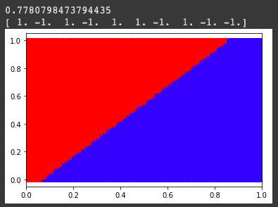
pred_ytrain=clf.predict(Xtest)
plt.xlim(0,1)
for i in range(len(pred_ytrain)):
if(pred_ytrain[i]==1):
clr='red'
if(pred_ytrain[i]==-1):
clr='blue'
plt.scatter(Xtest[i,0],Xtest[i,1],c=clr)
Output:
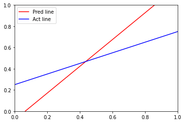
Visualizing original and logistic boundary
x_points = np.linspace(0,1,1000)

# Defining and plotting the predicted line
y_pred = -(clf.coef_[0][0]*x_points + clf.intercept_[0])/clf.coef_[0][1]
plt.xlim(0,1)
plt.ylim(0,1)
plt.plot(x_points, y_pred,'-r', label = 'Pred line')


y_act = (0.5*x_points + 0.25)
plt.plot(x_points, y_act, '-b', label = 'Act line')
plt.legend()
Output :
SVM function from scratch
def svm_function(x, y, epoch, l_rate):

    # Appending a fixed bias of +1 to all the datapoints
    list_X = x.tolist()
    for i in range(len(x)):
      list_X[i].append(1)
    x = np.asarray(list_X)

    # Initializing the weight vector with zeros
    w = np.zeros(len(x[0]))
    print(w.shape,x[1].shape)

    # Updating the weight vector
    for val in range(1,epoch):
        for i, point in enumerate(x):
            if (y[i]*np.dot(x[i], w)) < 1:
                w = w + l_rate * ((x[i]*y[i]) + (-2*(1/epoch)* w))
            else:
                w = w + l_rate * (-2*(1/epoch)* w)
    return w
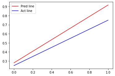
Train the dataset
data = np.asarray(data)
X = data[:,:2]
Y = data[:,2]
w = svm_function(X, Y, 10000, 1)

# plotting SVM vs original bounary
x_points = np.linspace(0,1,1000)


y_pred = (-w[0]*x_points - w[2])/w[1]
plt.plot(x_points, y_pred,'-r', label = 'Pred line')

# Defining and plotting the actual line
y_act = (0.5*x_points + 0.25)
plt.plot(x_points, y_act, '-b', label = 'Act line')
plt.legend()
Output:
Visualizing Decision boundary
X1=X[:,0]
X2=X[:,1]


def mapping(X1, X2):
  x = np.c_[(X1, X2)]
  #x_1 = x[:,0]**2
  #x_2 = np.sqrt(2)*x[:,0]*x[:,1]
  #x_3 = x[:,1]**2
  features_x = np.array([X1, X2])
  return features_x

features_x = mapping(X1, X2)


# Calling the previously defined SVM function
w =  svm_function(features_x.T, Y, 10000, 1)
The mapping function which is defined above is a no use here since we know that boundary is linear. But for nonlinear boundaries, the mapping function is of at most importance. To explain to you how to apply it for non-linear boundary, I have created the dataset link which will be given at the end of the session.
Visualizing the SVM boundary
def vis_dec_bnd():

  X1space = np.linspace(np.min(X1), np.max(X1), 100)
  X2space = np.linspace(np.min(X2), np.max(X2), 100)


  Xtest = []
  for i in range(100):
    for j in range(100):
      Xtest.append([X1space[i],X2space[j]])
  Xtest = np.asarray(Xtest)


  features_x = mapping(Xtest[:,0], Xtest[:,1]).T

  # Adding a column of all ones to match with the dimension of weight vector
  features_x = np.c_[features_x,np.ones(len(features_x))]

  # Classifying the points with trained SVM function
  for i in range(len(features_x)):
    if np.dot(features_x[i], w) > 0:
      plt.scatter(Xtest[i,0], Xtest[i,1], c = "r")
    else:
      plt.scatter(Xtest[i,0], Xtest[i,1], c = "b")
  return None


vis_dec_bnd()
Output:
Now using the same functions defined above we will try to visualize the non linear boundary.
Nonlinear dataset
import csv
with open('https://raw.githubusercontent.com/premssr/SVM-nonlinear-dataset/master/Csv1.csv', 'r') as f:
  values_csv2 = list(csv.reader(f, delimiter=','))


for x, y, l in values_csv2:
    if (int(l) == 1):
      clr = 'red'
    else:
      clr = 'blue'
    plt.scatter(float(x), float(y), c=clr)
Training and Visualization of non-linear dataset
X = []
Y = []

for row in values_csv2:
  X.append(row[:-1])
  Y.append(row[-1])

X = np.array(X).astype('float64')
Y = np.array(Y).astype('float64')

X1 = X[:,0]
X2 = X[:,1]

def mapping(X1, X2):
  x = np.c_[(X1, X2)]
  x_1 = x[:,0]
  x_2 = pow(x[:,0], 2)/0.4 + pow(x[:,1], 2)/0.8
  x_3 = x[:,1]
  features_x = np.array([X1, X2, x_1, x_2, x_3])
  return features_x

features_x = mapping(X1, X2)


w = svm_function(features_x.T, Y, 10000, 1)
print(w)


vis_dec_bnd()
Here is the link for the complete code and dataset https://github.com/premssr/SVM-nonlinear-dataset
That’s it guys we have applied two different algorithms on the same dataset and also observed how SVM is efficient in classifying nonlinear dataset. Please do comment if you could come up with a more efficient way to visualize the power of SVM.
Leave a Reply