scipy stats.cosine() in Python

By Vikrant Dey

The SciPy library comes with many variables to facilitate users to explore the world of statistics. One such variable is the scipy stats.cosine() variable in Python which we are going to discuss today. It is a continuous random variable with a standard format. Also, its definition needs some shape parameters.

So first, let us see what are the parameters of this variable. These are x, q, loc, scale, size, and moments:

• x (array) – number of quantiles.
• q (array) –  lower or upper-end probability.
• loc (array) – location parameter. The default is 0.
• scale (array) – scale parameter. The default is 1.
• size (int/tuple of ints) – the shape of random variables.
• moments (string) – composed of letters [‘mvsk’] specifying the moments to compute. Here, ‘m’, ‘v’, ‘s’, and ‘k’ are ‘mean’, ‘variance’, ‘(Fisher’s) skew’, and ‘(Fisher’s) kurtosis’. The default is ‘mv’.

Before we see the usage of this function, let us find out what it stands for. So, the cosine distribution approximates the normal distribution. Its probability density function is given by:

where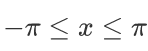 

Random Variates

Let us look at the random variates so that we can understand the basic functions.

from scipy.stats import cosine 
print(cosine.rvs(scale = 2,  size = 5))

Output:

[ 2.63039544 -1.80921027 -1.34999499 -4.21529217  1.33511733]

Probability Distribution

Let us have a look at how to generate a cosine distribution mentioning quantile, location, and scale.

import numpy as np
from scipy.stats import cosine 

quantile = np.arange (0.05, 1, 0.2) 
print(cosine.pdf(quantile, loc = 0, scale = 1))

Output:

[0.31811098 0.31336214 0.30246555 0.28585561 0.26419452]

Plotting the Distribution

Let us plot a cosine distribution.

import numpy as np
import matplotlib.pyplot as plt  
from scipy.stats import cosine 

dist = np.linspace(-1, np.minimum(cosine().dist.b, 4)) 
print(dist) 
  
plot = plt.plot(dist, cosine().pdf(dist))

Output:

[-1.         -0.9154777  -0.8309554  -0.7464331  -0.6619108  -0.5773885
 -0.49286621 -0.40834391 -0.32382161 -0.23929931 -0.15477701 -0.07025471
  0.01426759  0.09878989  0.18331219  0.26783449  0.35235678  0.43687908
  0.52140138  0.60592368  0.69044598  0.77496828  0.85949058  0.94401288
  1.02853518  1.11305748  1.19757978  1.28210207  1.36662437  1.45114667
  1.53566897  1.62019127  1.70471357  1.78923587  1.87375817  1.95828047
  2.04280277  2.12732506  2.21184736  2.29636966  2.38089196  2.46541426
  2.54993656  2.63445886  2.71898116  2.80350346  2.88802576  2.97254806
  3.05707035  3.14159265]

Hence. the diagram above plots the distribution printed above. As you can notice, the values range from -1 to ‘pi’.

Plotting Cosine and Stepfilled Distributions together

from scipy.stats import cosine
import numpy as np
import matplotlib.pyplot as plt

fig, ax = plt.subplots(1, 1)

mean, var, skew, kurt = cosine.stats(moments='mvsk')

l = np.linspace(cosine.ppf(0.02), cosine.ppf(0.9), 100))
ax.plot(l, cosine.pdf(l), 'r-', lw=10, alpha=0.6, label='cosine pdf')
ax.plot(l, cosine().pdf(l), lw=2, label='frozen pdf')

nums = cosine.ppf([0.001, 0.5, 0.9])
np.allclose([0.001, 0.5, 0.9], cosine.cdf(nums))

d = cosine.rvs(size=100)
ax.hist(d, density=True, histtype='stepfilled', alpha=0.5)
ax.legend(loc='best', frameon=False)

plt.show()

Output:

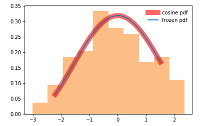
As discussed earlier, the cosine distribution is actually an approximation of the normal distribution. Hence the illustration above legitimizes the claim. If you want to bring changes in the manner of the visualization, you can easily do that. Though this is optional.

So this concludes a simplified tutorial on the scipy stats.cosine() variable in python. But a lot of work is still on you as you have to decide what parameters to use as per the problem statement.