Predict Weather Report Using Machine Learning in Python
 By Balender Singh
In this tutorial, we will learn how to predict the weather report using machine learning in python. In layman terms, I can simply define it as forecasting weather so I have used Time series forecasting to predict future values based on previously observed values.
Time series are widely used for non-stationary data, like economic data, weather reports, stock price, and retail sales. Let’s get started!
Predict Weather Report Using Machine Learning in Python
We are using Delhi weather data that can be downloaded from here.
Step 1:
Importing libraries
import pandas as pd #Data manipulation and analysis
import numpy as np  #It is utilised a number of mathematical operations
import seaborn as sn  #visualization
import matplotlib.pyplot as plt #plotting library
from datetime import datetime

import statsmodels.api as sm #Conducting statistical tests
from statsmodels.tsa.arima_model import ARIMA
from statsmodels.tsa.stattools import adfuller, acf, pacf
from statsmodels.graphics.tsaplots import plot_acf, plot_pacf
import pmdarima as pm #Statistical library
Step 2:
Importing dataset
The downloaded dataset is to be placed in the directory
df = pd.read_csv('delhi.csv')
Overview of the data
df.info()
<class 'pandas.core.frame.DataFrame'>
RangeIndex: 100990 entries, 0 to 100989
Data columns (total 20 columns):
 #   Column        Non-Null Count   Dtype
---  ------        --------------   -----
 0   datetime_utc  100990 non-null  object
 1    _conds       100918 non-null  object
 2    _dewptm      100369 non-null  float64
 3    _fog         100990 non-null  int64
 4    _hail        100990 non-null  int64
 5    _heatindexm  29155 non-null   float64
 6    _hum         100233 non-null  float64
 7    _precipm     0 non-null       float64
 8    _pressurem   100758 non-null  float64
 9    _rain        100990 non-null  int64
 10   _snow        100990 non-null  int64
 11   _tempm       100317 non-null  float64
 12   _thunder     100990 non-null  int64
 13   _tornado     100990 non-null  int64
 14   _vism        96562 non-null   float64
 15   _wdird       86235 non-null   float64
 16   _wdire       86235 non-null   object
 17   _wgustm      1072 non-null    float64
 18   _windchillm  579 non-null     float64
 19   _wspdm       98632 non-null   float64
dtypes: float64(11), int64(6), object(3)
memory usage: 15.4+ MB
as we can see here we have 100990 entries and 20 columns
Now let’s see the name of the columns
df.columns
Index(['datetime_utc', ' _conds', ' _dewptm', ' _fog', ' _hail',
       ' _heatindexm', ' _hum', ' _precipm', ' _pressurem', ' _rain', ' _snow',
       ' _tempm', ' _thunder', ' _tornado', ' _vism', ' _wdird', ' _wdire',
       ' _wgustm', ' _windchillm', ' _wspdm'],
      dtype='object')
Step 3:
Pre-processing and EDA(exploratory data analysis)
now let’s look for the missing values first because missing values can influence our outcome.
plt.figure(figsize=(8,8))
sns.barplot(x = df.count()[:],y = df.count().index)
plt.xlabel('Non null values count')
plt.ylabel('features')
Text(0, 0.5, 'features')

Now we can see that there are missing values in every column so now we are going to consider only a few of the columns which seem important for our basic EDA
df = df.drop([' _dewptm',' _fog',' _hail',' _heatindexm',' _pressurem',' _precipm',' _rain',' _snow',' _thunder',' _tornado',' _vism',' _wdird',' _wdire',' _wgustm',' _windchillm',' _wspdm'],axis=1)
df.head()
| datetime_utc | _conds | _hum | _tempm | |
|---|---|---|---|---|
| 0 | 19961101-11:00 | Smoke | 27.0 | 30.0 |
| 1 | 19961101-12:00 | Smoke | 32.0 | 28.0 |
| 2 | 19961101-13:00 | Smoke | 44.0 | 24.0 |
| 3 | 19961101-14:00 | Smoke | 41.0 | 24.0 |
| 4 | 19961101-16:00 | Smoke | 47.0 | 23.0 |
Now we can see that the date-time column is not in the desired format. So first, we will convert it into the desired format (YYYY-MM-DD HH: MM) And then we will make that column the index of the data
df['datetime_utc'] = pd.to_datetime(df['datetime_utc'].apply(lambda x: datetime.strptime(x,"%Y%m%d-%H:%M").strftime("%Y-%m-%d %H:%M")))
df['datetime_utc'].head()
0   1996-11-01 11:00:00
1   1996-11-01 12:00:00
2   1996-11-01 13:00:00
3   1996-11-01 14:00:00
4   1996-11-01 16:00:00
Name: datetime_utc, dtype: datetime64[ns]
# as we can see on the above table datatime_utc is column so we have to convert this to index
df = df.set_index('datetime_utc',drop = True)
df.index.name = 'datetime'
df.info()
<class 'pandas.core.frame.DataFrame'>
DatetimeIndex: 100990 entries, 1996-11-01 11:00:00 to 2017-04-24 18:00:00
Data columns (total 3 columns):
 #   Column      Non-Null Count   Dtype
---  ------      --------------   -----
 0   condition   100918 non-null  object
 1   humidity    100233 non-null  float64
 2   temprature  100317 non-null  float64
dtypes: float64(2), object(1)
memory usage: 3.1+ MB
for easy understanding, we are going to change the names of the remaining columns
df = df.rename(index = str, columns={' _conds':'condition',' _hum':'humidity',' _tempm':'temperature'})
df.head()
| datetime_utc | condition | humidity | temperature | |
|---|---|---|---|---|
| 0 | 1996-11-01 11:00:00 | Smoke | 27.0 | 30.0 |
| 1 | 1996-11-01 12:00:00 | Smoke | 32.0 | 28.0 |
| 2 | 1996-11-01 13:00:00 | Smoke | 44.0 | 24.0 |
| 3 | 1996-11-01 14:00:00 | Smoke | 41.0 | 24.0 |
| 4 | 1996-11-01 16:00:00 | Smoke | 47.0 | 23.0 |
we have fixed the Index issue, name of the columns and changed the date-time formate.
let’s fix the null values now
df.isnull().sum()
condition      72
humidity      757
temperature   673
dtype: int64
we will use mean to replace missing values in humidity and temperature
df.fillna(df.mean(), inplace=True)
df.isnull().sum()
condition     72
humidity       0
temperature    0
dtype: int64
We have fixed the missing values of humidity and temperature, let’s fix the condition we have to use the front fit method for this Categorical variable
df.ffill(inplace=True)
df[df.isnull()].count()
condition     0
humidity      0
temprature    0
dtype: int64
let’s visualize conditions
weather_condition   = (df.condition.value_counts()/(df.condition.value_counts().sum())) * 100
weather_condition.plot.bar(figsize=(16,9))
plt.xlabel('Weather Conditions')
plt.ylabel('Percent')
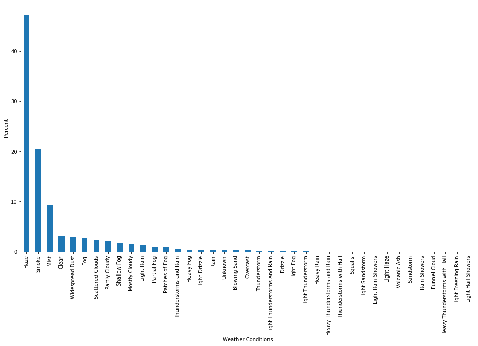
We can see that the weather condition mostly is haze and smoke this is all due to pollution
df = df.resample('H').mean().interpolate()
df.info()
<class 'pandas.core.frame.DataFrame'>
DatetimeIndex: 179504 entries, 1996-11-01 11:00:00 to 2017-04-24 18:00:00
Freq: H
Data columns (total 2 columns):
 #   Column       Non-Null Count   Dtype
---  ------       --------------   -----
 0   humidity     179504 non-null  float64
 1   temperature  179504 non-null  float64
dtypes: float64(2)
memory usage: 4.1 MB
We can see that the categorical variable condition is not here and the frequency is added to the Date-time index
Let’s find out outliers in our data. I have used here describe method to check for outliers we can also use box plot to identify
df.describe()
| humidity | temperature | |
|---|---|---|
| count | 179504.000000 | 179504.000000 |
| mean | 58.425165 | 25.065563 |
| std | 23.465756 | 8.266500 |
| min | 4.000000 | 1.000000 |
| 25% | 40.000000 | 19.000000 |
| 50% | 59.000000 | 26.867000 |
| 75% | 78.000000 | 31.000000 |
| max | 243.000000 | 90.000000 |
df = df[df.temperature < 50]
df = df[df.humidity <= 100]

df.describe()
| humidity | temperature | |
|---|---|---|
| count | 179488.000000 | 179488.000000 |
| mean | 58.422029 | 25.063841 |
| std | 23.452692 | 8.262075 |
| min | 4.000000 | 1.000000 |
| 25% | 40.000000 | 19.000000 |
| 50% | 59.000000 | 26.861713 |
| 75% | 78.000000 | 31.000000 |
| max | 100.000000 | 48.333333 |
df.plot(subplots = True , figsize= (15,6))
array([<matplotlib.axes._subplots.AxesSubplot object at 0x0000028B5410A248>,
       <matplotlib.axes._subplots.AxesSubplot object at 0x0000028B5412D8C8>],
      dtype=object)
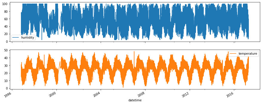
df['2015':'2016'].resample('D').fillna(method='pad').plot(subplots=True, figsize=(20,12))
array([<matplotlib.axes._subplots.AxesSubplot object at 0x0000028B54D87C08>,
       <matplotlib.axes._subplots.AxesSubplot object at 0x0000028B54F95648>],
      dtype=object)
![df['2015':'2016'].resample('D').fillna(method='pad').plot(subplots=True, figsize=(20,12))](https://www.codespeedy.com/wp-content/uploads/2020/04/04.png)
The humidity is lower between April and July and the temperature is greater in the mid two quarter
Step 4:
Let’s decompose the time series to visualize trend, season and noise separately
train = df[:'2015']
test = df['2016':]

def decomposeNplot(data):
  decomposition = sm.tsa.seasonal_decompose(data)

  plt.figure(figsize=(15,16))

  ax1 = plt.subplot(411)
  decomposition.observed.plot(ax=ax1)
  ax1.set_ylabel('Observed')

  ax2 = plt.subplot(412)
  decomposition.trend.plot(ax=ax2)
  ax2.set_ylabel('Trend')

  ax3 = plt.subplot(413)
  decomposition.seasonal.plot(ax=ax3)
  ax3.set_ylabel('Seasonal')

  ax4 = plt.subplot(414)
  decomposition.resid.plot(ax=ax4)
  ax4.set_ylabel('Residuals')

  return decomposition

# Resampling the data to mothly and averaging out the temperature & we will predict the monthly average temperature
ftraindata = train['temperature'].resample('M').mean()
ftestdata = test['temperature'].resample('M').mean()

# Taking the seasonal difference S=12 and decomposing the timeseries
decomposition = decomposeNplot(ftraindata.diff(12).dropna())

results = adfuller(ftraindata.diff(12).dropna())
results
(-3.789234435915501,
 0.0030194014111634623,
 14,
 203,
 {'1%': -3.462980134086401,
  '5%': -2.875885461947131,
  '10%': -2.5744164898444515},
 738.4331626389505)
p-value <= 0.05: Reject the null hypothesis (H0), the data does not have a unit root and is stationary
We observed before that there is a yearly periodic pattern -> Seasonal
To get non-seasonal orders of the SARIMAX Model we will first use ACF & PACF plots
plt.figure(figsize=(10,8))

ax1 = plt.subplot(211)
acf = plot_acf(ftraindata.diff(12).dropna(),lags=30,ax=ax1)

ax2 = plt.subplot(212)
pacf = plot_pacf(ftraindata.diff(12).dropna(),lags=30,ax=ax2)
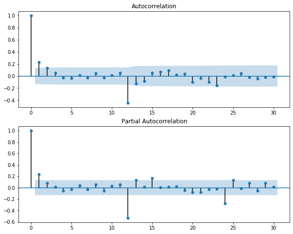
It's hard to get the idea of the non-seasonal orders from these plots
lags = [12*i for i in range(1,4)]

plt.figure(figsize=(10,8))

ax1 = plt.subplot(211)
acf = plot_acf(ftraindata.diff(12).dropna(),lags=lags,ax=ax1)

ax2 = plt.subplot(212)
pacf = plot_pacf(ftraindata.diff(12).dropna(),lags=lags,ax=ax2)

results = pm.auto_arima(ftraindata,seasonal=True, m=12,d=0,D=1,trace=True,error_action='ignore',suppress_warnings=True)
Performing stepwise search to minimize aic
Fit ARIMA: (2, 0, 2)x(1, 1, 1, 12) (constant=True); AIC=746.883, BIC=773.959, Time=5.936 seconds
Fit ARIMA: (0, 0, 0)x(0, 1, 0, 12) (constant=True); AIC=861.067, BIC=867.836, Time=0.063 seconds
Fit ARIMA: (1, 0, 0)x(1, 1, 0, 12) (constant=True); AIC=792.173, BIC=805.711, Time=0.519 seconds
Fit ARIMA: (0, 0, 1)x(0, 1, 1, 12) (constant=True); AIC=748.617, BIC=762.155, Time=2.779 seconds
Near non-invertible roots for order (0, 0, 1)(0, 1, 1, 12); setting score to inf (at least one inverse root too close to the border of the unit circle: 1.000)
Fit ARIMA: (0, 0, 0)x(0, 1, 0, 12) (constant=False); AIC=859.369, BIC=862.753, Time=0.059 seconds
Fit ARIMA: (2, 0, 2)x(0, 1, 1, 12) (constant=True); AIC=746.155, BIC=769.847, Time=4.267 seconds
Near non-invertible roots for order (2, 0, 2)(0, 1, 1, 12); setting score to inf (at least one inverse root too close to the border of the unit circle: 1.000)
Fit ARIMA: (2, 0, 2)x(1, 1, 0, 12) (constant=True); AIC=796.814, BIC=820.506, Time=2.523 seconds
Fit ARIMA: (2, 0, 2)x(2, 1, 1, 12) (constant=True); AIC=748.988, BIC=779.449, Time=14.277 seconds
Near non-invertible roots for order (2, 0, 2)(2, 1, 1, 12); setting score to inf (at least one inverse root too close to the border of the unit circle: 1.000)
Fit ARIMA: (2, 0, 2)x(1, 1, 2, 12) (constant=True); AIC=749.082, BIC=779.542, Time=14.701 seconds
Near non-invertible roots for order (2, 0, 2)(1, 1, 2, 12); setting score to inf (at least one inverse root too close to the border of the unit circle: 1.000)
Fit ARIMA: (2, 0, 2)x(0, 1, 0, 12) (constant=True); AIC=850.698, BIC=871.005, Time=1.009 seconds
Fit ARIMA: (2, 0, 2)x(0, 1, 2, 12) (constant=True); AIC=748.537, BIC=775.613, Time=15.565 seconds
Near non-invertible roots for order (2, 0, 2)(0, 1, 2, 12); setting score to inf (at least one inverse root too close to the border of the unit circle: 1.000)
Fit ARIMA: (2, 0, 2)x(2, 1, 0, 12) (constant=True); AIC=778.693, BIC=805.769, Time=3.744 seconds
Fit ARIMA: (2, 0, 2)x(2, 1, 2, 12) (constant=True); AIC=750.709, BIC=784.554, Time=12.544 seconds
Near non-invertible roots for order (2, 0, 2)(2, 1, 2, 12); setting score to inf (at least one inverse root too close to the border of the unit circle: 1.000)
Fit ARIMA: (1, 0, 2)x(1, 1, 1, 12) (constant=True); AIC=746.534, BIC=770.226, Time=3.604 seconds
Near non-invertible roots for order (1, 0, 2)(1, 1, 1, 12); setting score to inf (at least one inverse root too close to the border of the unit circle: 1.000)
Fit ARIMA: (2, 0, 1)x(1, 1, 1, 12) (constant=True); AIC=744.691, BIC=768.382, Time=3.829 seconds
Near non-invertible roots for order (2, 0, 1)(1, 1, 1, 12); setting score to inf (at least one inverse root too close to the border of the unit circle: 1.000)
Fit ARIMA: (3, 0, 2)x(1, 1, 1, 12) (constant=True); AIC=743.924, BIC=774.385, Time=2.851 seconds
Near non-invertible roots for order (3, 0, 2)(1, 1, 1, 12); setting score to inf (at least one inverse root too close to the border of the unit circle: 1.000)
Fit ARIMA: (2, 0, 3)x(1, 1, 1, 12) (constant=True); AIC=750.534, BIC=780.995, Time=3.040 seconds
Near non-invertible roots for order (2, 0, 3)(1, 1, 1, 12); setting score to inf (at least one inverse root too close to the border of the unit circle: 1.000)
Fit ARIMA: (1, 0, 1)x(1, 1, 1, 12) (constant=True); AIC=744.620, BIC=764.927, Time=1.428 seconds
Near non-invertible roots for order (1, 0, 1)(1, 1, 1, 12); setting score to inf (at least one inverse root too close to the border of the unit circle: 1.000)
Fit ARIMA: (1, 0, 3)x(1, 1, 1, 12) (constant=True); AIC=748.493, BIC=775.569, Time=1.454 seconds
Near non-invertible roots for order (1, 0, 3)(1, 1, 1, 12); setting score to inf (at least one inverse root too close to the border of the unit circle: 1.000)
Fit ARIMA: (3, 0, 1)x(1, 1, 1, 12) (constant=True); AIC=748.466, BIC=775.542, Time=1.826 seconds
Near non-invertible roots for order (3, 0, 1)(1, 1, 1, 12); setting score to inf (at least one inverse root too close to the border of the unit circle: 1.000)
Fit ARIMA: (3, 0, 3)x(1, 1, 1, 12) (constant=True); AIC=752.426, BIC=786.271, Time=2.774 seconds
Near non-invertible roots for order (3, 0, 3)(1, 1, 1, 12); setting score to inf (at least one inverse root too close to the border of the unit circle: 1.000)
Total fit time: 98.833 seconds
Fitting the ARIMA model
mod = sm.tsa.statespace.SARIMAX(ftraindata,
                                order=(3, 0, 3),
                                seasonal_order=(1, 1, 1, 12),
                                enforce_stationarity=False,
                                enforce_invertibility=False)

results = mod.fit()
print(results.summary())
 SARIMAX Results
============================================================================================
Dep. Variable:                          temperature   No. Observations:                  230
Model:             SARIMAX(3, 0, 3)x(1, 1, [1], 12)   Log Likelihood                -338.758
Date:                              Thu, 16 Apr 2020   AIC                            695.515
Time:                                      16:54:34   BIC                            725.290
Sample:                                  11-30-1996   HQIC                           707.562
                                       - 12-31-2015
Covariance Type:                                opg
==============================================================================
                 coef    std err          z      P>|z|      [0.025      0.975]
------------------------------------------------------------------------------
ar.L1          0.1548      1.185      0.131      0.896      -2.168       2.477
ar.L2          0.5894      0.494      1.192      0.233      -0.380       1.558
ar.L3         -0.3190      0.596     -0.535      0.593      -1.487       0.849
ma.L1          0.2347      1.193      0.197      0.844      -2.103       2.573
ma.L2         -0.5308      0.936     -0.567      0.570      -2.365       1.303
ma.L3          0.2525      0.346      0.730      0.465      -0.425       0.930
ar.S.L12      -0.0585      0.091     -0.644      0.520      -0.237       0.120
ma.S.L12      -0.8759      0.088     -9.918      0.000      -1.049      -0.703
sigma2         1.4823      0.202      7.337      0.000       1.086       1.878
===================================================================================
Ljung-Box (Q):                       38.72   Jarque-Bera (JB):                20.19
Prob(Q):                              0.53   Prob(JB):                         0.00
Heteroskedasticity (H):               0.53   Skew:                            -0.23
Prob(H) (two-sided):                  0.01   Kurtosis:                         4.48
===================================================================================

Warnings:
[1] Covariance matrix calculated using the outer product of gradients (complex-step).
let’s diagnose the results
results.plot_diagnostics(figsize=(16, 8))
plt.show()

Here we can see:
Standardized residual plot: No obvious structure ✔
Histogram & KDE: KDE is normally distributed ✔
Normal Q-Q: Almost all the points are on the red line ✔
Correlogram of residuals: is nearly zero for all lags ✔
Mean Absolute Error for training data
print(np.mean(np.abs(results.resid)))
forecast = results.get_forecast(steps=len(ftestdata))
predictedmean = forecast.predicted_mean
bounds = forecast.conf_int()
lower_limit = bounds.iloc[:,0]
upper_limit = bounds.iloc[:,1]
plt.figure(figsize=(15,7))

plt.plot(ftraindata.index, ftraindata, label='train')
plt.plot(ftestdata.index,ftestdata,label='actual')

plt.plot(predictedmean.index, predictedmean, color='r', label='forecast')

plt.fill_between(lower_limit.index,lower_limit,upper_limit, color='pink')

plt.xlabel('Date')
plt.ylabel('Delhi Temperature')
plt.legend()
plt.show()

#Producing and visualizing forecast

pred_uc = results.get_forecast(steps=100)
pred_ci = pred_uc.conf_int()
ax = ftraindata.plot(label='observed', figsize=(14, 7))
pred_uc.predicted_mean.plot(ax=ax, label='Forecast')
ax.fill_between(pred_ci.index,
                pred_ci.iloc[:, 0],
                pred_ci.iloc[:, 1], color='k', alpha=.25)
ax.set_xlabel('Date')
ax.set_ylabel('Delhi Temprature')
plt.legend()
plt.show()

Step 6:
Saving the model for future reference
import joblib

joblib.dump(forecast,'finalized_model.pkl')
Hello, can you please predict weather report using random forest and decision three algorithms in one project?