Machine Learning | Customer Churn Analysis Prediction

Hello folks!

In this article, we are going to see how to build a machine learning model for Customer Churn analysis Prediction. Basically customer churning means that customers stopped continuing the service. There are various machine learning algorithms such as logistic regression, decision tree classifier, etc which we can implement for this.

Also, there are various datasets available online related to Customer churn. For this article, we are going to use a dataset from Kaggle: https://www.kaggle.com/blastchar/telco-customer-churn.

In this dataset there are both categorical features and numerical futures, so we will use the Pipeline from sklearn for the same and apply the Decision Tree Classifier learning algorithm for this problem.

Customer Churn Analysis Prediction Code in Python

We will write this code in Google Colab for better understanding and handling. See the code below:

from google.colab import files
uploaded = files.upload()
import pandas as pd
import io
df = pd.read_csv(io.BytesIO(uploaded['WA_Fn-UseC_-Telco-Customer-Churn.csv']))
df = df[~df.duplicated()] # remove duplicates
total_charges_filter = df.TotalCharges == " "
df = df[~total_charges_filter]
df.TotalCharges = pd.to_numeric(df.TotalCharges)

Here we first upload our data and then read that data in a CSV file using pandas.

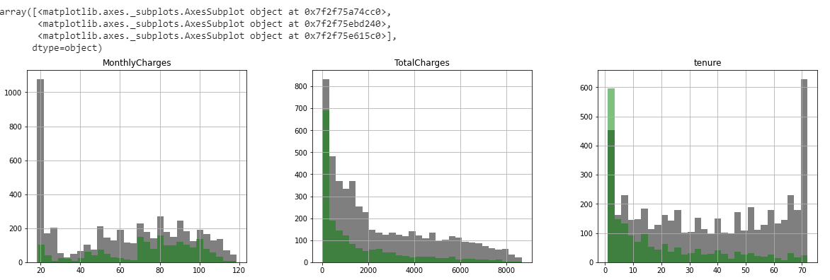
categoric_features = [
 "DeviceProtection","InternetService","gender","OnlineSecurity","OnlineBackup","TechSupport","StreamingTV",
 "StreamingMovies","Contract","PaperlessBilling","SeniorCitizen","Partner","Dependents","PhoneService","MultipleLines",
 "PaymentMethod",
]
numeric_features = [ "MonthlyCharges","tenure", "TotalCharges"]
output = "Churn"
df[numerical_features].hist(bins=40, figsize=(7,7 ),color="green")

Then we will divide the data into categoric_features and numeric_features present in the CSV file. And plot the histogram of numeric data.

import matplotlib.pyplot as plt
fig, ax = plt.subplots(1, 3, figsize=(20, 5))
df[df.Churn == "No"][numerical_features].hist(bins=30, color="black", alpha=0.5, ax=ax)
df[df.Churn == "Yes"][numerical_features].hist(bins=30, color="green", alpha=0.5, ax=ax)

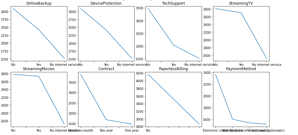
R, C = 4, 4
fig, ax = plt.subplots(R, C, figsize=(18, 18))
row, col = 0, 0
for i, categorical_feature in enumerate(categorical_features):
    if col == C - 1:
        row += 1
    col = i % C
    df[categorical_feature].value_counts().plot(x='bar', ax=ax[row, col]).set_title(categorical_feature)

from sklearn.pipeline import Pipeline
from sklearn.preprocessing import OneHotEncoder

categorical_transformer = Pipeline(steps=[
    ('onehot', OneHotEncoder(handle_unknown='ignore')),
])
from sklearn.impute import SimpleImputer
from sklearn.preprocessing import StandardScaler

numeric_transformer = Pipeline(steps=[
    ('imputer', SimpleImputer(strategy='median')),
    ('scaler', StandardScaler()),
])
from sklearn.compose import ColumnTransformer

preprocessor = ColumnTransformer(
    transformers=[
        ('num', numeric_transformer, numerical_features),
        ('cat', categorical_transformer, categorical_features)
    ]
)
from sklearn import tree

clf = Pipeline([
     ('preprocessor', preprocessor),
     ('clf', tree.DecisionTreeClassifier(max_depth=3,random_state=42))

Then we will import our python sklearn library to make a pipeline for combining categoric and numerical features together and apply them to the decision tree model.

from sklearn.model_selection import train_test_split
df_train, df_test = train_test_split(df, test_size=0.20, random_state=42)
clf.fit(df_train, df_train[output])
prediction = clf.predict(df_test)

from sklearn.metrics import classification_report
print(classification_report(df_test[output], prediction)

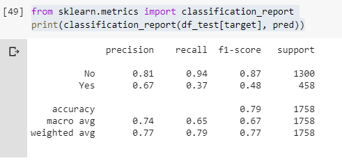
Then we will split our data into training and testing set. And give our training set to pipeline “calf” to train our model. After this, we will print out our results on the screen that you can see in the image above.

I hope you enjoyed the article. Thank you!