Logistic Regression from scratch in Python

By Sakshi Gawande

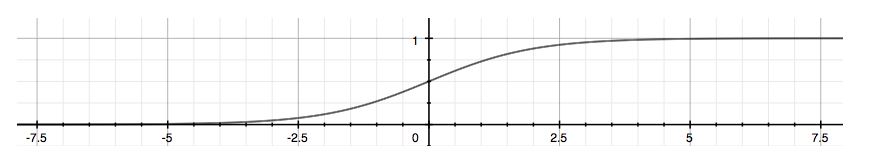
Classification techniques are used to handle categorical variables. Logistic Regression is a linear classifier which returns probabilities(P(Y=1) or P(Y=0)) as a function of the dependent variable(X).The dependent variable is a binary variable that contains data in the form of either success(1) or failure(0).

Let’s say we want to predict for a person, knowing their age, whether he will take up the offer or not. The offer is ‘to purchase a Lenovo 800 mobile model’.How about instead we will state a probability or a likelihood of that person taking that offer.

It is the same way we find a line or a formula for a curve that best fits our data. Thel loss function, which is the sigmoid function f(x) is used to map any real number to the (0, 1) interval.

f(x)=1/(1+e^(-z))

The graph for the sigmoid function is shown below:

Prerequisites for implementing the code:

1. Your system must have a Spyder(Python 3.7) or any other latest version software installed.
2. You need to have a dataset file, which is generally an ms-excel file, with a .csv extension.
3. Set the folder as a working directory, in which your dataset is stored.
4. You need to have a basic understanding of  Python programming language.

Step by step implementation:

Make sure that you check the prerequisites before proceeding. Also, your system should be efficient and lag-free.

1. Importing the libraries:

Firstly, let us import the necessary libraries.

import numpy as np
import matplotlib.pyplot as plt
import pandas as pd

2. Importing the dataset

The dataset is as shown below:

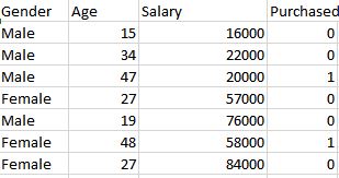
dataset = pd.read_csv('lenovo 800_customers.csv')
X = dataset.iloc[:, [2, 3]].values
y = dataset.iloc[:, 4].values

3. Deciding the training and the test set

from sklearn.model_selection import train_test_split 
X_trainset, X_testset, y_trainset, y_testset = train_test_split(X, y, test_size = 0.25, random_state = 0)

4. Feature Scaling

from sklearn.preprocessing import StandardScaler
ss = StandardScaler()
X_trainset = ss.fit_transform(X_trainset)
X_testset = ss.transform(X_testset)

5. Fitting Logistic Regression to the Training set

from sklearn.linear_model import LogisticRegression
classifier = LogisticRegression(random_state = 0)
classifier.fit(X_trainset, y_trainset)

6. Predicting the Test set results

The confusion matrix is a  simple  Matrix with two rows, two columns that will show us the number of correct predictions we did. Interestingly, it will show us the results for both the type of customers, i.e. those who purchased and those who didn’t.

y_pred = classifier.predict(X_testset)
from sklearn.metrics import confusion_matrix
cm = confusion_matrix(y_testset, y_pred)

7. Plotting the Test set results

Finally, we can best understand the concept of logistic regression through the following plot:

from matplotlib.colors import ListedColormap
X_set, y_set = X_testset, y_testset
X1, X2 = np.meshgrid(np.arange(start = X_set[:, 0].min() - 1, stop = X_set[:, 0].max() + 1, step = 0.01),
                     np.arange(start = X_set[:, 1].min() - 1, stop = X_set[:, 1].max() + 1, step = 0.01))
plt.contourf(X1, X2, classifier.predict(np.array([X1.ravel(), X2.ravel()]).T).reshape(X1.shape),
             alpha = 0.75, cmap = ListedColormap(('orange', 'blue')))
plt.xlim(X1.min(), X1.max())
plt.ylim(X2.min(), X2.max())
for i, j in enumerate(np.unique(y_set)):
    plt.scatter(X_set[y_set == j, 0], X_set[y_set == j, 1],
                c = ListedColormap(('orange', 'blue'))(i), label = j)
plt.title('Test set')
plt.xlabel('Age')
plt.ylabel('Salary')
plt.legend()
plt.show()

So, you can clearly spot incorrect predictions with the respective colors.

Conclusion:

As we can clearly see from the plot, we get a straight line for linear models. We can use the model to test on similar datasets with more number of independent variables.