Image Classification using Keras in TensorFlow Backend

Step 3: Preprocessing Input and Output

We need to Normalise our data values to a range between 0 and 1. For this, we divide the data values by 255 since we know that the maximum RGB value is 255. But before this, we need to convert the data type to float32.

xtrain=xtrain.astype('float32')
xtest=xtest.astype('float32')
xtrain/=255
xtest/=255

Also, to process the y-array, we need to convert the 1D array with 10 classes to 10 arrays with one class each. The 10 classes correspond to 10 categories.

ytrain=np_utils.to_categorical(ytrain,10)
ytest=np_utils.to_categorical(ytest,10)
print(ytrain.shape)
print(ytest.shape)

Output:

(50000, 10)
(10000, 10)

Step 4: Creating the network

First, we need to define the model. Since we are making a sequential model, we create a Sequential model object.

m = Sequential()

Next, we need to add the input convolution layer (CNN) using Conv2D. The first parameter ie.32 represents the number of filters and (3,3) represents the number of rows and columns. The input_shape is the shape of one input image ie. (32,32,3)

m.add(Conv2D(32,(3,3),activation='relu',input_shape=xtrain.shape[1:]))

We can add as many CNNs in between as we want.

m.add(Conv2D(32,(3,3),activation='relu'))
m.add(MaxPooling2D(pool_size=(2,2)))
m.add(Dropout(0.2))

To know more about Conv2D, MaxPooling, Dropout etc, visit Keras documentation
Next, we add the Fully connected Dense layers. Make sure that the outputs from CNN are flattened before feeding it to the dense layers.

m.add(Flatten())
m.add(Dense(512,activation='relu'))
m.add(Dropout(0.5))

Then, add the final output layer. The first Parameter in Dense is the number of outputs. So, the final layer has 10 outputs corresponding to 10 categories.

m.add(Dense(10, activation='softmax'))

With this, we have completed our network.

Step 5: Compiling, Training, Evaluating

The compile() method defines a loss function, optimizer (we have used predefined ‘Adadelta’), and metrics. You need to compile a model before training.

m.compile(loss='categorical_crossentropy',optimizer='adadelta',metrics=['accuracy'])

The fit () method trains the data using the training inputs. We have defined the batch_size as 32 and epochs as 2. Epoch is the number of passes over the entire dataset. Higher the Epoch, the higher will be the accuracy. I have only used 2 because higher values require a lot of time and resources. For this dataset, at least 50 datasets are required to get good accuracy.

m.fit(xtrain,ytrain,batch_size=32,epochs=2)

Output:

Epoch 1/2
50000/50000 [==============================] - 178s 4ms/step - loss: 0.9548 - accuracy: 0.6668
Epoch 2/2
50000/50000 [==============================] - 185s 4ms/step - loss: 0.8568 - accuracy: 0.7028

The evaluate() method is used after you have trained your model. It takes the testing inputs and outputs loss and accuracy.

result = m.evaluate(xtest, ytest)
print(result)

Output:

10000/10000 [==============================] - 9s 919us/step
[0.8568861591339111, 0.7028000273704529]

Step 6: Predicting

Evaluate() and predict() are not the same. Predict() outputs the category for the given input data. Thus we pass the testing inputs as parameters. It outputs an (n x 10) array containing the probabilities of each category(column) for that particular image(row).

ypred = m.predict(xtest)
print(ypred)

Output:

[[1.52685883e-04 1.60379231e-03 3.51585657e-03 ... 1.31038280e-04
  6.27783127e-03 2.18168786e-03]
 [1.11513287e-02 8.53282690e-01 7.34639571e-07 ... 3.84769594e-09
  1.27586797e-01 7.97820278e-03]
  ...
 [2.13376582e-02 8.15662503e-01 2.58647744e-03 ... 2.49057682e-03
  5.43371600e-04 3.23010795e-03]
 [1.04555793e-05 1.44058195e-05 9.92649235e-04 ... 9.27792609e-01
  2.97331007e-06 1.92014850e-05]]

Alternatively,
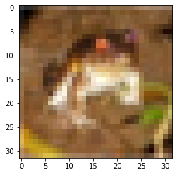
We can choose a particular index and predict the image as follows:

x=int(input("Enter the index of any picture from the test batch to predict ie. enter a number from 1 to 10000:  "))
print("\nPrediction: \n",ypred[x])
print("\nActual: \n",ytest[x])
plt.imshow(xtest[x])

Output:

Enter the index of any picture from the test batch to predict ie. enter a number from 1 to 10000:  6000

Prediction: 
 [0.08831886 0.05823785 0.08399942 0.03805733 0.0353229  0.00504771
 0.01562174 0.00598332 0.47863427 0.19077668]

Actual: 
 [0. 0. 0. 0. 0. 0. 0. 0. 1. 0.]

<matplotlib.image.AxesImage at 0x1d9dc984488>

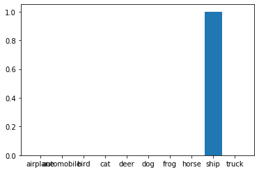
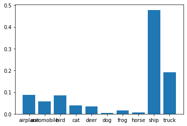
Let’s plot a graph of the actual and the predicted probabilities:

labels=['airplane','automobile','bird','cat','deer','dog','frog','horse','ship','truck']

plt.bar(labels,ytest[x])                          # actual
plt.bar(labels,ypred[x])                          # predicted

Output: 

Actual:-

<BarContainer object of 10 artists>

            Prediction:

<BarContainer object of 10 artists>

 

Image Classification using Keras requires a lot of time and computation power. If you are lacking both, you can use Nanonets API: visit Image classification using Nanonets API in Python