Image Augmentation Using skimage in Python

By Amal Mathew

In this tutorial, we will learn about image augmentation using skimage in Python. The size of the dataset used while training a deep learning /machine learning model significantly impacts its performance. Therefore to have a dataset with a huge size poses a high priority while training the model as it can affect the accuracy of the model directly. But to create a huge dataset is very difficult considering the size should be in the order of gigabytes. This is where image augmentation plays a vital role, with a limited amount of images (data)  augmenting images create a multitude of images from a single image thereby creating a large dataset.

There are different techniques like rotation, flipping, shifting, etc which are used in transforming the image to create new images. The size of the dataset will raise in the power of 10 with just four, five types of transformation techniques. Python library such as NumPy and skimage makes it easy for augmenting images.

There are two ways of augmenting an image:

1. Positional Augmentation
   In this type of image augmentation, the input image is transformed on the basis of pixel positions. Only the relative positions of each pixel are changed in order to transform the image. Some of the various positional augmentation techniques involved are Scaling, rotation, cropping, flipping, padding, zoom, translation, shearing, and other affine transformations.
2. Colour Augmentation
   In this type of image augmentin technique, the intensity of the image pixels are tweaked and configured on the basis of brightness, saturation, contrast.

Various Image Augmentation with Python code example

First, we need to import basic libraries for augmenting

from skimage import transform
from skimage.transform import rotate, AffineTransform,warp
from skimage.util import random_noise
from skimage.filters import gaussian
from scipy import ndimage
import random
from skimage import img_as_ubyte
import os

#basic Function to display image side by side
def plot_side(img1, img2, title1, title2, cmap = None):
    fig = plt.figure(tight_layout='auto', figsize=(10, 7))
    fig.add_subplot(221)
    plt.title(title1)
    plt.imshow(img)

    fig.add_subplot(222)
    plt.title(title2)
    plt.imshow(img2, cmap = None)
    return fig

Next, we load and display the Original image

# load Image
img = imread('./flower.jpg') / 255
# plot original Image
plt.imshow(img)
plt.title('Original')
plt.show()

The Output:

Image Rotation

# image rotation using skimage.transformation.rotate
rotate30 = rotate(img, angle=30)
rotate45 = rotate(img, angle=45)
rotate60 = rotate(img, angle=60)
rotate90 = rotate(img, angle=90)
fig = plt.figure(tight_layout='auto', figsize=(10, 10))
fig.add_subplot(221)
plt.title('Rotate 30')
plt.imshow(rotate30)
fig.add_subplot(222)
plt.title('Rotate 45')
plt.imshow(rotate45)
fig.add_subplot(223)
plt.title('Rotate 60')
plt.imshow(rotate60)
fig.add_subplot(224)
plt.title('Rotate 90')
plt.imshow(rotate90)
plt.show()

Output:

Image Shearing

# image shearing using sklearn.transform.AffineTransform
# try out with differnt values of shear 

tf = AffineTransform(shear=-0.5)
sheared = transform.warp(img, tf, order=1, preserve_range=True, mode='wrap')
sheared_fig = plot_side(img, sheared, 'Original', 'Sheared')

Output:

Warp transformation

#Affine Transformation(warping)

transform = AffineTransform(translation=(-200,0)) 
 
# (-200,0) are x and y coordinate, change it see the effect
warp_image = warp(img,transform, mode="wrap") #mode parameter is optional
# mode= {'constant', 'edge', 'symmetric', 'reflect', 'wrap'}
#these are possible values of mode, you can try them and decide 
#which one to use, default value for mode is constant
warp_fig = plot_side(img,warp_image , 'Original', 'Wrap image')

Output:

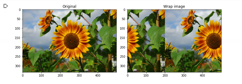
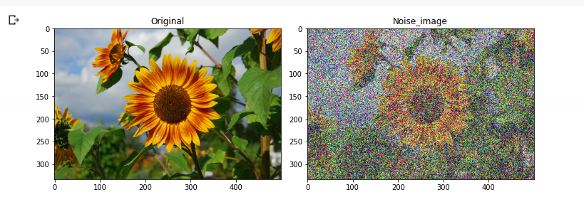
Image Noising

#image Noising

noisy_image = random_noise(img, var=0.1**.01)
noise_fig = plot_side(img,noisy_image , 'Original', 'Noise_image')

Output:

Blurring

#image Blurring

from scipy import ndimage
blured_image = ndimage.uniform_filter(img, size=(11, 11, 1))

noise_fig = plot_side(img,blured_image , 'Original', 'Blurred')

Output:

Increasing Brightness

# Increasing the brighness of the Image
# Note: Here we add 100/255 since we scaled Intensity values of 
#Image when loading (by dividing it 255)

highB = img + (100/255)
fig_highB = plot_side(img, highB, 'Original', 'Brightened')
plt.show()

Output:

Up-Down Flipping

# flip up-down using np.flipud

up_down = np.flipud(img)
fig_updown = plot_side(img, up_down, 'Original', 'Up-Down')
plt.show()

Output:

Increasing Contrast

# Increasing the contrast of the Image
# Note: Here we add 100/255 since we scaled Intensity 
#values of Image when loading (by dividing it 255)
highC = img * 3

fig_highB = plot_side(img, highC, 'Original', 'highContast')
plt.show()

Output:

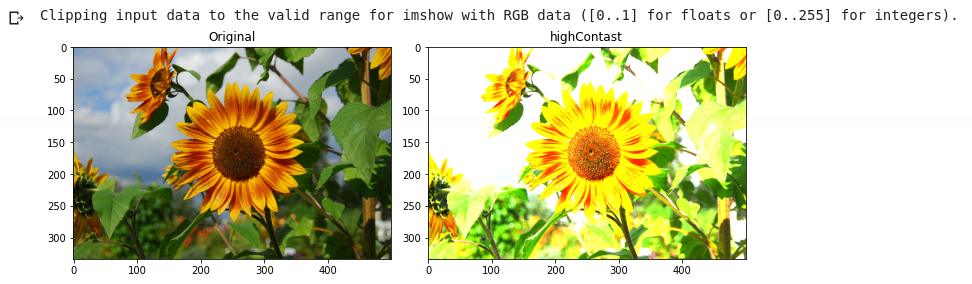
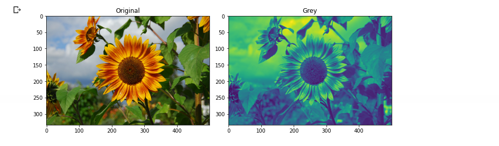
Image Greyscaling

#GreyScale

from skimage.color import rgb2gray

gray_scale_image = rgb2gray(img)
Grey = plot_side(img,gray_scale_image , 'Original', 'Grey')
plt.show()

Output:

Gamma Correction

import numpy as np
from skimage import exposure

v_min, v_max = np.percentile(img, (0.2, 99.8))
better_contrast = exposure.rescale_intensity(img, in_range=(v_min, v_max))
contrast = plot_side(img,better_contrast , 'Original', 'Better_contrast')
plt.show()

#Gamma correction
adjusted_gamma_image = exposure.adjust_gamma(img, gamma=0.4, gain=0.9)
gamma = plot_side(img,better_contrast , 'Original', 'gamma_exposure')
plt.show()

Output:

Color Inversion

from skimage import util
import numpy as np

color_inversion = util.invert(img)
gamma = plot_side(img,color_inversion , 'Original', 'Inversion')
plt.show()

Output:

We can write the new images onto the disk, or we can use this in Keras pipelines to augment while reading the data.
I hope it was helpful. Let me know if you have any critics or have a way to improve it.