Gradient Descendent – A Minimization Technique in Python

By Praveen Kumar

In this tutorial, We are going to understand a minimization technique in machine Learning called Gradient Descendent. This is an optimization algorithm that finds a minimum of functions that can be local or global. In this task, we are going to use Python as the programming language.

What we actually do is make a point and starts moving towards minima. It’s like we at some height of the hill and moves downward i.e. along the negative gradient. We will move downward direction till we get a point which cannot further be minimized.

The main objective for doing all these to minimize the cost function.

A cost function is actually a mathematical relationship between cost and output. It tells how costs change in response to changes in the output.

Function and its Derivatives

We have the following equation for Simple Linear Regression:

Y = X² + X + 1

We have original function, f(x) = X² + X + 1
And its Derivatives of function df(x) = 2*X + 1

Below is Implementation in Python:

#Our Original Function
def f(x):
    return x**2 + x + 1

#Function for derivatives for function
def df(x):
    return 2*x + 1

Method

Now let’s see how this method works.

Pre-Requisite: Python

Steps for getting a minimum of a function:

Step 1:

Start with a random point say 3, then find the gradient (derivative) of the given function.

Step 2:

We start to move in the direction of negative of gradients.

But how much to move, for that we need to define Learning Rate.

Learning rate is a hyper-parameter that can control how much we are adjusting the weights of the network with respect to the loss gradient. It helps us of making sure that we do not miss any local minima.

new_weight = existing_weight — learning_rate * gradient

In our code, we define it as step_multiplier

# Gradient Descent
new_x = 3
previous_x = 0
step_multiplier = 0.1
precision = 0.00001

x_list = [new_x]
slope_list = [df(new_x)]

for n in range(500):
    previous_x = new_x
    gradient = df(previous_x)
    new_x = previous_x - step_multiplier * gradient
    
    step_size = abs(new_x - previous_x)
#     print(step_size)
    
    x_list.append(new_x)
    slope_list.append(df(new_x))
    
    if step_size < precision:
        print('Loop ran this many times:', n)
        break
    
print('Local minimum occurs at:', new_x)
print('Slope or df(x) value at this point is:', df(new_x))
print('f(x) value or cost at this point is:', f(new_x))

Output:

Loop ran this many times: 50

Local minimum occurs at: -0.49996003706460423

Slope or df(x) value at this point is: 7.992587079153068e-05

f(x) value or cost at this point is: 0.7500000015970362

Now we can see that loop ran only for 50 times instead of 500 iterations. This is because we introduced precision = 0.00001, which is the objective of using precision is to make sure of best minima in a way of controlling iteration count.

In other words, if the difference between new_X and prev_X  is getting very close than we understand that we reached local minima. So when we get the difference less than precision then we come out of the loop.

However precision is not mandatory for performing minimization but if we can have a measure for precision then we actually get minima in fewer iterations. In other words, if we once reached minima then we cannot have further minima for further iterations.

Let’s see how its steps changing for each iteration. Also, we can see how X is decreasing each iteration.

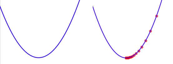
The left one image is the graph for the original equation. And the image at the right side is showing how its step size and value for X is changing initialized from X=3 till reaching minima of the function.