Generative Adversarial Network (GAN) in Python – TensorFlow
 By Kartheek Janapati
In this lecture we will learn about Generative Adversarial Network (GAN) using Python.
What is a Generative Adversarial Network (GAN)?
A Generative Adversarial Network is basically a framework to train generative models. It comprises two neural networks: a generator and a discriminator. In essence, this means a generator comes up with artificial data samples, while a discriminator is trained to distinguish between real and fake samples. The two networks are trained at the same time in a process where the generator is getting better at the creation of realistic data and the discriminator is becoming more perfect at the detection of fake data.
Types of GANs
Vanilla GAN: This can be said to be one of the very first GANs, proposed by Goodfellow et al. in the year 2014.
Conditional GAN: Here, it is a variant of GAN that uses extra information like labels to generate data.
DCGAN: Deep Convolutional GAN for Image Generation.
CycleGAN: This allows for image-to-image translation without paired examples.
StyleGAN: Generates images with controllable styles and attributes.
Progressive GAN: It generates high-resolution images due to progressive resolution during training.
WGAN: This uses a different loss function to hopefully improve training stability.
Architecture of GANs
There are Two components in GAN
- Generator
- Discriminator
Generator
- Takes random noise as an input.
- Transforms the noise into a data sample.
- It could be an image, for instance. Normally, it employs a few layers like fully connected, convolutional, in case of image, and batch normalization layers.
Also check Optical Character recognition using Deep Learning (CNN)
Discriminator
- Takes a data sample as an input. This may either be real or fake in nature.
- The output will also give the probability of whether the input is real or a fake one.
- Normally employs convolutional layers, for instance, when dealing with images, dropout layers, and fully connected layers.
How does a GAN work?
- Noise Input: Random noise is the input to a generator.
- Generated Data: It serves as noise from which generators can create data samples.
- Input to Discriminator: Real data from the dataset; fake data coming from the generator.
- Discriminator Output: It gives back a likelihood score for every sample, telling whether it is real or fake.
- Adversarial Training:
The discriminator strives to maximize the accuracy of telling the real apart from the fake.
The generator strives to reduce the capability of the discriminator in classifying fake samples correctly. Through such adversarial processes, it keeps running until the generator can output data which cannot be differentiated from real data.
Implementation of a GAN
Step 1: Import Libraries
import tensorflow as tf
from tensorflow.keras import layers
import matplotlib.pyplot as plt

# Load the dataset
(train_images, _), (_, _) = tf.keras.datasets.mnist.load_data()
train_images = train_images.reshape(train_images.shape[0], 28, 28, 1).astype('float32')
train_images = (train_images - 127.5) / 127.5  # Normalize to [-1, 1]
BUFFER_SIZE = 60000
BATCH_SIZE = 256
train_dataset = tf.data.Dataset.from_tensor_slices(train_images).shuffle(BUFFER_SIZE).batch(BATCH_SIZE)
output :
Downloading data from https://storage.googleapis.com/tensorflow/tf-keras-datasets/mnist.npz 11490434/11490434 [==============================] – 0s 0us/step
Step 2: Create the Generator
def make_generator_model():
    model = tf.keras.Sequential([
        layers.Dense(7*7*256, use_bias=False, input_shape=(100,)),
        layers.BatchNormalization(),
        layers.LeakyReLU(),
        layers.Reshape((7, 7, 256)),
        layers.Conv2DTranspose(128, (5, 5), strides=(1, 1), padding='same', use_bias=False),
        layers.BatchNormalization(),
        layers.LeakyReLU(),
        layers.Conv2DTranspose(64, (5, 5), strides=(2, 2), padding='same', use_bias=False),
        layers.BatchNormalization(),
        layers.LeakyReLU(),
        layers.Conv2DTranspose(1, (5, 5), strides=(2, 2), padding='same', use_bias=False, activation='tanh')
    ])
    return model

generator = make_generator_model()
Step 3: Create the Discriminator
def make_discriminator_model():
    model = tf.keras.Sequential([
        layers.Conv2D(64, (5, 5), strides=(2, 2), padding='same', input_shape=[28, 28, 1]),
        layers.LeakyReLU(),
        layers.Dropout(0.3),
        layers.Conv2D(128, (5, 5), strides=(2, 2), padding='same'),
        layers.LeakyReLU(),
        layers.Dropout(0.3),
        layers.Flatten(),
        layers.Dense(1)
    ])
    return model

discriminator = make_discriminator_model()
Step 4: Define Loss and Optimizers
cross_entropy = tf.keras.losses.BinaryCrossentropy(from_logits=True)

def discriminator_loss(real_output, fake_output):
    real_loss = cross_entropy(tf.ones_like(real_output), real_output)
    fake_loss = cross_entropy(tf.zeros_like(fake_output), fake_output)
    total_loss = real_loss + fake_loss
    return total_loss

def generator_loss(fake_output):
    return cross_entropy(tf.ones_like(fake_output), fake_output)

generator_optimizer = tf.keras.optimizers.Adam(1e-4)
discriminator_optimizer = tf.keras.optimizers.Adam(1e-4)
Step 5: Training Loop
EPOCHS = 4  # Reduced to 4 epochs
noise_dim = 100
num_examples_to_generate = 16
seed = tf.random.normal([num_examples_to_generate, noise_dim])

@tf.function
def train_step(images):
    noise = tf.random.normal([BATCH_SIZE, noise_dim])

    with tf.GradientTape() as gen_tape, tf.GradientTape() as disc_tape:
        generated_images = generator(noise, training=True)

        real_output = discriminator(images, training=True)
        fake_output = discriminator(generated_images, training=True)

        gen_loss = generator_loss(fake_output)
        disc_loss = discriminator_loss(real_output, fake_output)

    gradients_of_generator = gen_tape.gradient(gen_loss, generator.trainable_variables)
    gradients_of_discriminator = disc_tape.gradient(disc_loss, discriminator.trainable_variables)

    generator_optimizer.apply_gradients(zip(gradients_of_generator, generator.trainable_variables))
    discriminator_optimizer.apply_gradients(zip(gradients_of_discriminator, discriminator.trainable_variables))

def generate_and_save_images(model, epoch, test_input):
    predictions = model(test_input, training=False)

    fig = plt.figure(figsize=(4, 4))

    for i in range(predictions.shape[0]):
        plt.subplot(4, 4, i + 1)
        plt.imshow(predictions[i, :, :, 0] * 127.5 + 127.5, cmap='gray')
        plt.axis('off')

    plt.savefig('image_at_epoch_{:04d}.png'.format(epoch))
    plt.show()

def train(dataset, epochs):
    for epoch in range(epochs):
        for image_batch in dataset:
            train_step(image_batch)

        # Produce images for the GIF as we go
        generate_and_save_images(generator, epoch + 1, seed)

        print(f'Epoch {epoch+1} completed')

train(train_dataset, EPOCHS)
Output:

Epoch 1 completed
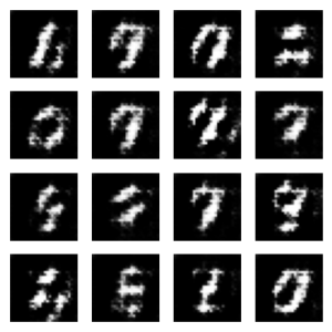
Epoch 2 completed
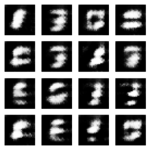
Epoch 3 completed
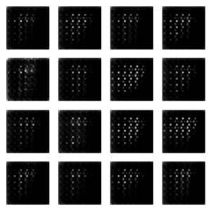
Epoch 4 completed
Application of Generative Adversarial Networks (GANs)
- Image Generation: The generation of realism from random noise images; for instance, the generation of face and artistic images.
- Image-to-Image Translation: Domains are translated into images; for instance, sketches to photos and day to night.
- Text-to-Image Synthesis: It basically generates images from textual descriptions.
- Super-Resolution: The resolution of an image can be enhanced.
- Data Augmentation: It generates other training data for supervised learning machine learning models.
- Medical Imaging: Medical image generation for better diagnosis and enhancement.
Advantages of GAN
- High-Quality Data Generation: The important strength of GANs are that they generate high-quality data that seems near real.
- Varied Applications: From artificial image synthesis to data augmentation, the applications are very diverse.
- Adversarial Nature for Continuous Improvisation: Because of the adversarial nature, there will be continuous improvisation on both the generator and the discriminator.
Disadvantages of GAN
- Training Instability: Training can be unstable and sensitive to hyperparameters.
- Mode Collapse: The generator seed into a mode of producing a limited variety of outputs.
- Resource-Intensive: This process is very resource-intensive in computational time and power.
- Challenges in the Evaluation: The quality and diversity of the generated data are very hard to assess, be it one or the other
Leave a Reply