Facial expression detection using Machine Learning in Python
 By Priya Bansal
Ever wondered, what if your camera could tell you the state of your mind based on its interpretation of your facial expression? Facial expression detection using Machine Learning in Python has made it possible.
A meaningful piece of code can do wonders. In this tutorial, we will implement facial expression detection using machine learning in Python.
Data set: Facial Expression Detection, Source: Kaggle. The entire script has two sections: for training and for testing the model.
Facial expression detection using ML
Before we jump to the code, there are a few prerequisites. For implementing this code, one must have to install NumPy, pandas, openCV-Python, TensorFlow, and Keras.
You can do so by:
pip install numpy
pip install pandas
pip install openCV-python
pip install keras
pip install tensorflow
Code Section 1: Training our model
Moving on to our code, we start with importing certain libraries into our Python notebook. I have executed my code on Google colaboratory as it is comparatively faster than jupyter notebook. But, for successful implementation in one go, I would recommend using jupyter notebook.
import os
import keras
from __future__ import print_function
from keras.preprocessing.image import ImageDataGenerator
from keras.layers import Dense,Dropout,Activation,Flatten,BatchNormalization,Conv2D,MaxPooling2D
from keras.models import Sequential
from keras.optimizers import RMSprop,SGD,Adam
from keras.callbacks import ModelCheckpoint, EarlyStopping, ReduceLROnPlateau
Importing OS module- to allow our code to interact with the Operating System. Imported keras – an open source neural network library which is basically written in the Python language, and can easily run on top of TensorFlow. From Keras, import the rest of the modules – to enable our code to perform various functions.
no_of_classes = 5                      #classes are - angry, sad, surprised, happy, neutral, count = 5
SIZEbatch = 32                         #each batch in our data set contains 32 images
imageROWS,imageCOLUMNS = 48,48         #target size is 48 by 48
Since I have used google colaboratory to implement this code, I’m importing my data set from my google drive. If you have downloaded the data set on your desktop, you can directly access it by specifying the path.
from google.colab import drive

drive.mount('/content/gdrive', force_remount=True)
Now we are proceeding towards the data augmentation step, where we will use the module ImageDataGenerator to give specifications as follows:
training_training = ImageDataGenerator(
          width_shift_range=0.4,
          height_shift_range=0.4,
          horizontal_flip=True,
          fill_mode='nearest'
          rescale=1./255,
          rotation_range=30,
          shear_range=0.3,
          zoom_range=0.3,)
In this step
we are giving the parameters for normalizing each pixel of our image, and to what extent we would like to rotate our image starting from 0 degrees. Note that these specifications or parameters apply to our training data set only. To know more about each of these parameters under the ImageDataGenerator module, kindly visit ImageDataGenerator keras.
For the validation data set, only this particular normalization specification can suffice, as we do not require as many images for validation as we require to train our model:
validating_validating = ImageDataGenerator(rescale=1./255)
Next, we have to take the data frame and the path of our data set (here the path is from my drive) into a directory and then generate or develop batches of augmented or normalized data using the above data. And to do so, the flow_from_directory method and its specifications are employed as follows:
trainGenerator = training_training.flow_from_directory(
          'gdrive/My Drive/fer2013/train',
          color_mode='grayscale',
          target_size=(imageROWS,imageCOLUMNS),
          batch_size=SIZEbatch,
          class_mode='categorical',
          shuffle=True)

output : Found 24256 images belonging to 5 classes.
Grayscale – because we don’t require colors to classify our emotions. The class mode is categorical as we have multiple classes (5 here). Shuffle is set to true because the model needs appropriate training. To understand the use of each specification under flow_of_directory, visit: Image preprocessing keras.
The above steps contain the generation of our training data set. Similarly, for the validation data set :
validGenerator = validating_validating.flow_from_directory(
              'gdrive/My Drive/fer2013/validation',
              color_mode='grayscale',
              target_size=(imageROWS,imageCOLUMNS),
              batch_size=SIZEbatch,
              class_mode='categorical',
              shuffle=True)

output: Found 3006 images belonging to 5 classes.
Incorporating Convolutional Neural Network into our model
Now we specify our model type which is sequential as we want to add everything layer-by-layer.
model=sequential()
Moving on to neural networks, its time to employ the Conv2D, Activation, BatchNormalization, Dropout, MaxPooling2D modules under the keras.layers to train our model conveniently.
Here comes blocks of code to activate the neurons in the neural network. These are similar but the only difference is that, with each subsequent block the number of neurons doubles. This process shall start with our batch size that is 32 in #part1 and 64 in #part2 and so on until the desired number of neurons to be activated is achieved.
The model.add() method comes in use here. 3 by 3 matrices of specified neurons are being made with uniform padding throughout. ‘he_normal’ is set as it gives good variance for the distribution in terms of statistics. ‘elu’ activation – so it doesn’t have negative values and gives more accuracy. Dropout refers to the percentage of neurons to be left out or deactivated during transmission at one time. MaxPooling2D – for dimensionality reduction while BatchNormalization calculates the linear function in layers.
#part1

model.add(Conv2D(32,(3,3),padding='same',kernel_initializer='he_normal',input_shape=(imageROWS,imageCOLUMNS,1))) #input_shape is to be specified only once
model.add(Activation('elu'))       #using elu as it doesn't have negative input and smoothes slowly
model.add(BatchNormalization())
model.add(Conv2D(32,(3,3),padding='same',kernel_initializer='he_normal',input_shape=(imageROWS,imageCOLUMNS,1)))
model.add(Activation('elu'))
model.add(BatchNormalization())
model.add(MaxPooling2D(pool_size=(2,2)))
model.add(Dropout(0.2))    #dropout refers to the percentage of neurons to be deactivated while transmission
#part2

model.add(Conv2D(64,(3,3),padding='same',kernel_initializer='he_normal'))
model.add(Activation('elu'))
model.add(BatchNormalization())
model.add(Conv2D(64,(3,3),padding='same',kernel_initializer='he_normal'))
model.add(Activation('elu'))
model.add(BatchNormalization())
model.add(MaxPooling2D(pool_size=(2,2)))
model.add(Dropout(0.2))
#part3

model.add(Conv2D(128,(3,3),padding='same',kernel_initializer='he_normal'))
model.add(Activation('elu'))
model.add(BatchNormalization())
model.add(Conv2D(128,(3,3),padding='same',kernel_initializer='he_normal'))
model.add(Activation('elu'))
model.add(BatchNormalization())
model.add(MaxPooling2D(pool_size=(2,2)))
model.add(Dropout(0.2))
#part4

model.add(Conv2D(256,(3,3),padding='same',kernel_initializer='he_normal'))
model.add(Activation('elu'))
model.add(BatchNormalization())
model.add(Conv2D(256,(3,3),padding='same',kernel_initializer='he_normal'))
model.add(Activation('elu'))
model.add(BatchNormalization())
model.add(MaxPooling2D(pool_size=(2,2)))
model.add(Dropout(0.2))
Specifying the ‘input_shape’ is one time job, as the subsequent part will adjust in accordance with the output of the preceding part.
The Convolutional Neural Network part of our code ends here.
Its time to flatten our matrices and get into the dense layer.
We use the ‘Conv’ layer for associating a feature with its neighboring features, and ‘dense’ layer for associating each feature to every other feature. ‘Flatten’ plays the role of adjusting the format to pass on to the dense layer. These connections play an important role when it comes to object detection.
#part1
model.add(Flatten())
model.add(Dense(64,kernel_initializer='he_normal'))
model.add(Activation('elu'))
model.add(BatchNormalization())
model.add(Dropout(0.5))

#part2
model.add(Dense(64,kernel_initializer='he_normal'))
model.add(Activation('elu'))
model.add(BatchNormalization())
model.add(Dropout(0.5))

#part3
model.add(Dense(no_of_classes,kernel_initializer='he_normal'))
model.add(Activation('softmax'))
Instead of ‘elu’, ‘softmax’ is given, because we want to analyze our output as a probability distribution.
Output 1: Let’s see what we have done so far
print(model.summary())

#output:

Model: "sequential_2"
_________________________________________________________________
Layer (type)                 Output Shape              Param #
=================================================================
conv2d_9 (Conv2D)            (None, 48, 48, 32)        320
_________________________________________________________________
activation_12 (Activation)   (None, 48, 48, 32)        0
_________________________________________________________________
batch_normalization_11 (Batc (None, 48, 48, 32)        128
_________________________________________________________________
conv2d_10 (Conv2D)           (None, 48, 48, 32)        9248
_________________________________________________________________
activation_13 (Activation)   (None, 48, 48, 32)        0
_________________________________________________________________
batch_normalization_12 (Batc (None, 48, 48, 32)        128
_________________________________________________________________
max_pooling2d_5 (MaxPooling2 (None, 24, 24, 32)        0
_________________________________________________________________
dropout_7 (Dropout)          (None, 24, 24, 32)        0
_________________________________________________________________
conv2d_11 (Conv2D)           (None, 24, 24, 64)        18496
_________________________________________________________________
activation_14 (Activation)   (None, 24, 24, 64)        0
_________________________________________________________________
batch_normalization_13 (Batc (None, 24, 24, 64)        256
_________________________________________________________________
conv2d_12 (Conv2D)           (None, 24, 24, 64)        36928
_________________________________________________________________
activation_15 (Activation)   (None, 24, 24, 64)        0
_________________________________________________________________
batch_normalization_14 (Batc (None, 24, 24, 64)        256
_________________________________________________________________
max_pooling2d_6 (MaxPooling2 (None, 12, 12, 64)        0
_________________________________________________________________
dropout_8 (Dropout)          (None, 12, 12, 64)        0
_________________________________________________________________
conv2d_13 (Conv2D)           (None, 12, 12, 128)       73856
_________________________________________________________________
activation_16 (Activation)   (None, 12, 12, 128)       0
_________________________________________________________________
batch_normalization_15 (Batc (None, 12, 12, 128)       512
_________________________________________________________________
conv2d_14 (Conv2D)           (None, 12, 12, 128)       147584
_________________________________________________________________
activation_17 (Activation)   (None, 12, 12, 128)       0
_________________________________________________________________
batch_normalization_16 (Batc (None, 12, 12, 128)       512
_________________________________________________________________
max_pooling2d_7 (MaxPooling2 (None, 6, 6, 128)         0
_________________________________________________________________
dropout_9 (Dropout)          (None, 6, 6, 128)         0
_________________________________________________________________
conv2d_15 (Conv2D)           (None, 6, 6, 256)         295168
_________________________________________________________________
activation_18 (Activation)   (None, 6, 6, 256)         0
_________________________________________________________________
batch_normalization_17 (Batc (None, 6, 6, 256)         1024
_________________________________________________________________
conv2d_16 (Conv2D)           (None, 6, 6, 256)         590080
_________________________________________________________________
activation_19 (Activation)   (None, 6, 6, 256)         0
_________________________________________________________________
batch_normalization_18 (Batc (None, 6, 6, 256)         1024
_________________________________________________________________
max_pooling2d_8 (MaxPooling2 (None, 3, 3, 256)         0
_________________________________________________________________
dropout_10 (Dropout)         (None, 3, 3, 256)         0
_________________________________________________________________
flatten_2 (Flatten)          (None, 2304)              0
_________________________________________________________________
dense_4 (Dense)              (None, 64)                147520
_________________________________________________________________
activation_20 (Activation)   (None, 64)                0
_________________________________________________________________
batch_normalization_19 (Batc (None, 64)                256
_________________________________________________________________
dropout_11 (Dropout)         (None, 64)                0
_________________________________________________________________
dense_5 (Dense)              (None, 64)                4160
_________________________________________________________________
activation_21 (Activation)   (None, 64)                0
_________________________________________________________________
batch_normalization_20 (Batc (None, 64)                256
_________________________________________________________________
dropout_12 (Dropout)         (None, 64)                0
_________________________________________________________________
dense_6 (Dense)              (None, 5)                 325
_________________________________________________________________
activation_22 (Activation)   (None, 5)                 0
=================================================================
Total params: 1,328,037
Trainable params: 1,325,861
Non-trainable params: 2,176
_________________________________________________________________
None
Great, we have our model functioning well. We will now use checkpoint to save what we’ve done into the file specified (you can replace ‘FileName’ with your filename) so that we can resume from this point for further fitting and evaluation. In this step, we’ll try to minimize the loss or simply keep a check on it. EarlyStopping prevents overfitting and ‘reduceLRonplateau’ is for reducing the rate of learning once the model has achieved the desired accuracy.
Check_pointing = ModelCheckpoint('FileName.h5',
                             monitor='val_loss',
                             mode='min',
                             save_best_only=True,
                             verbose=1)
Early_stop = EarlyStopping(monitor='val_loss',
                          min_delta=0,
                          patience=3,
                          verbose=1,
                          restore_best_weights=True
                          )
ReducingLR = ReduceLROnPlateau(monitor='val_loss',
                              factor=0.2,
                              patience=3,
                              verbose=1,
                              min_delta=0.0001)
Once these parameters have been given, we can now use callbacks to get a complete view of the internal states of our training model. This step will be followed by model.compile() as we need a loss function and optimizer for training the model.
callbacks = [Early_stop,Check_pointing,ReducingLR]

model.compile(loss='categorical_crossentropy',
              optimizer = Adam(lr=0.001),
              metrics=['accuracy'])

trainSAMPLES = 24176  #this number is generated as the output of trainGenerator step
validSAMPLES = 3006   #this number is generated as the output of valid Generator step
EpocH=10

Final_step=model.fit_generator(
                train_generator,
                steps_per_epoch=trainSAMPLES//SIZEbatch,
                epochs=EpocH,
                callbacks=callbacks,
                validation_data=validGenerator,
                validation_steps=validSAMPLES//SIZEbatch)
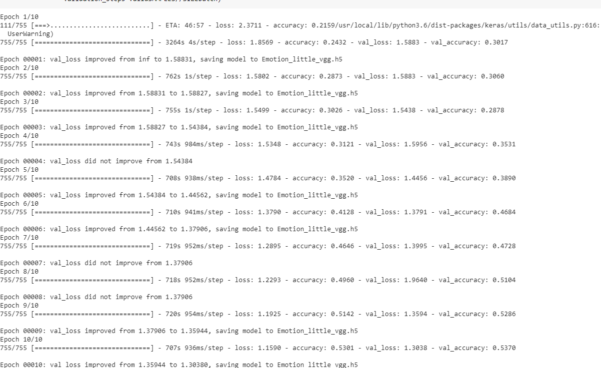
Epoch is an important term, it determines how many times the code will iterate to achieve considerable accuracy. Lastly, declare the Final_step which employs model.fit_generator() method to work upon training our model by utilizing whatever we achieved until now.
I took epoch=10 here, so it took a couple of hours to execute.
You could take a higher value for the epoch to achieve better accuracy.
Output 2:
Eventually, the output will be ready, and it will look as follows:
Code Section 2: Testing our model
Remember check_pointing? Yes, the file where we saved everything for later use is now to be used.
We’ll be using OpenCV for opening the camera, load_model module from Keras to load the saved model, image module to load the image, img_to_array module from Keras to convert the images into an array, and finally the sleep module from time for required delays.
import numpy
import cv2
from time import sleep
from keras.models import load_model
from keras.preprocessing import image
from keras.preprocessing.image import img_to_array
Loading the test data set
from google.colab import drive

drive.mount('/content/gdrive', force_remount=True)
The inception of the process takes place by letting our classifier detect a face in its frame. For this we’ll be using CascadeClassifier() method and load_model() method.
FACEclass = cv2.CascadeClassifier('haarcascade_frontalface_default.xml')
Clas =load_model('FileName.h5')
Now we’ll add labels to our classes (expression name) in alphabetical order
labelCLASS = ['Angry','Happy','Neutral','Sad','Surprise']
What next?
What will happen when your camera comes across a face? It will locate the face, convert it to a grayscale image, get it into a single frame, and then as per its training and metrics, it will evaluate and produce the desired result.
To achieve this, I’ve used the following methods in my code:
- detectMultiScale() to reduce the width and height of the image for faster execution
- cvtColor() to convert to grayscale
- rectangle() to specify the dimensions and color of the rectangular frame
- resize() and INTER_AREA to fit as per our metrics of the image
- astype() for normalizing with specified data type
- expand_dims() to expand the dimension of the input shape as per the axis value
- argmax() to find the class with the highest value of predicted probability.
- putText() to allow the overlay of our text onto the image
- imshow() to optimize the figure and the properties of the image
- waitKey() to wait for the user to press any key
- waitKey(1) & 0xff=ord(‘q’) are for binary calculations which result in breaking of the loop in case any key is pressed.
I have provided short descriptions in the code snippet to make it easily comprehensible.
#Opens your camera
click = cv2.VideoCapture(0)

#LOGIC:
while True:
    RT, FramE = click.read()  #getting a frame
    LabeLs = []                #empty list for labels
    colorGRAY = cv2.cvtColor(FramE,cv2.COLOR_BGR2GRAY)     #converting image to gray scale
    FACE = FACEclass.detectMultiScale(gray,1.3,5)        #getting coordinates

    for (i,j,k,l) in FACE:       #i,j,k,l represent the dimensions of the rectangular frame
        cv2.rectangle(FramE,(i,j),(i+k,j+l),(255,0,0),2)
        RO_colorGRAY = colorGRAY[j:j+l,i:i+k]
        RO_colorGRAY = cv2.resize(RO_colorGRAY,(48,48),interpolation=cv2.INTER_AREA)

        if numpy.sum([RO_colorGRAY])!=0:  #execute this block if there is atleast one face

            RO = RO_colorGRAY.astype('float')/255.0    #Normalizing the frame from the webcam
            RO = img_to_array(RO)
            RO = numpy.expand_dims(RO,axis=0)
        # predicting on the desired region and making classes
            Prediic = Clas.predict(RO)[0]
            LabeL=labelCLASS[Prediic.argmax()]
            positionLABEL = (i,j)
            cv2.putText(FramE,LabeL,positionLABEL,cv2.FONT_HERSHEY_DUPLEX,2,(0,255,0),3)  #specifying how to present the text
        #In case the face couldn't be detected or there is no face
        else:
            cv2.putText(FramE,'Where are you?',(20,60),cv2.FONT_HERSHEY_DUPLEX,2,(0,255,0),3)
    cv2.imshow('Recognizing your Expression',FramE)
    if cv2.waitKey(1) & 0xFF == ord('q'):
        break
This is the end of code section 2.
Output 3: It was all worth it, The final result

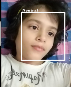
This is an example- how to go about facial expression detection using machine learning techniques in Python language. To learn more about the methods, modules and parameters used in the code you can visit: Keras Conv2D with examples in Python.
Leave a Reply