Data Analysis for multidimensional data in Python

By Premkumar Vemula

In this article, we will explore the sequential steps needed to perform while handling the multidimensional data to use it in Machine Learning Algorithm with Python code implementation.

There are many issues to be faced while handling Multidimensional data like missing data, collinearity, multicollinearity, categorical attributes etc. Let see how to deal with each one of them.

Link to the dataset and code will be provided at the end of the article.

Data Analysis

Import Data

import pandas as pd
sheet=pd.read_csv("https://raw.githubusercontent.com/premssr/Steps-in-Data-analysis-of-Mutidimensional-data/master/Train_before.csv")
sheet.head()

Output:

Understanding Data

sheet.describe(include='all')

Output:

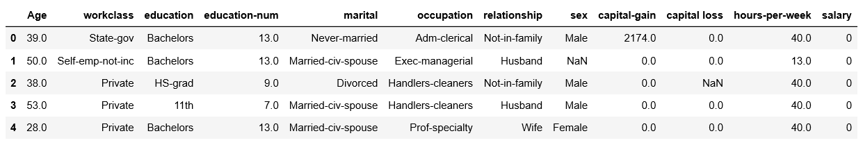
There are some numerical and some categorical predictors in this data. Salary column is the one we need to predict we first convert the column into variables 0 or 1. This thing has been done as the first step of data analysis in our CSV file itself. Now the given data has some missing.

Divide the predictors and response

pdytrain=sheet['salary']
pdxtrain=sheet.drop('salary',axis=1)
pdxtrain.head()

Output :

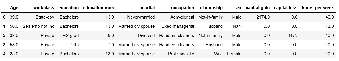
Generally, when we collect data in practice there are some missing values. This might be attributed to the negligence of volunteer who is collecting data for us or to miss the inefficient design of the experiment. Whatever the reason is we The Data Analyst have to cope up with it. There are quite a few methods to handle it. If we have enough data that removal of the data points won’t affect our model then we go for it. Otherwise, we replace the missing value with appropriate value mean, median or mode of the attribute. This method is called Imputation. We will replace the missing value with most frequent (mode) in the case of discrete attributes and with mean in case of continuous attributes.

Count number of missing data from each attribute

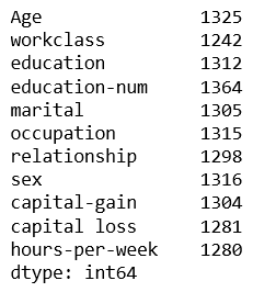
pdxtrain.isnull().sum()

Output:

Imputation

from sklearn.impute import SimpleImputer

npxtrain=np.array(pdxtrain)
npytrain=np.array(pdytrain)

#for categories
imp = SimpleImputer(missing_values=np.nan, strategy='most_frequent')
imp.fit(npxtrain[:,[1,2,4,5,6,7]])
pred_categ=imp.transform(npxtrain[:,[1,2,4,5,6,7]])


#for continuos

imp = SimpleImputer(missing_values=np.nan, strategy='mean')
imp.fit(npxtrain[:,[0,3,8,9,10]])
pred_int=imp.transform(npxtrain[:,[0,3,8,9,10]])

npimputedxtrain=np.c_[pred_categ,pred_int]
pdimputedxtrain=pd.DataFrame(npimputedxtrain)

pdimputedxtrain.columns =['workclass', 'education','marital status','occupation','relationship','sex','Age','education-num','capital-gain',
             'capital loss','hours-per-week']

pdimputedxtrain.describe(include='all')

Output:

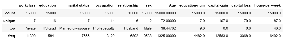
Now once we have whole set of data. We will now convert discrete data to a binary value of 0 or 1. This is called One Hot Encoding. But for categorical data we fir label encode them that is replace categories with numbers then go for one hot encoding.

Lebel Encoding

from sklearn.preprocessing import OneHotEncoder
from sklearn.preprocessing import LabelEncoder

le = LabelEncoder() 
  
pdimputedxtrain['workclass']= le.fit_transform(pdimputedxtrain['workclass']) 
pdimputedxtrain['education']= le.fit_transform(pdimputedxtrain['education'])
pdimputedxtrain['marital status']= le.fit_transform(pdimputedxtrain['marital status'])
pdimputedxtrain['occupation']= le.fit_transform(pdimputedxtrain['occupation'])
pdimputedxtrain['relationship']= le.fit_transform(pdimputedxtrain['relationship'])
pdimputedxtrain['sex']= le.fit_transform(pdimputedxtrain['sex'])




pdimputedxtrain=pdimputedxtrain.drop(['education'],axis=1)
print(pdimputedxtrain.head())




pdOneHotencoded.columns =['Federal-gov', 'Local-gov', 'Private', 'Self-emp-not-inc','State-gov','Self-emp-inc','Without-pay','Married-AF-        spouse','Married-civ-spouse','Married-spouse-absent','Divorced','Never-married','Separated','Widowed','cater','Adm-clerical',' Armed-Forces',' Exec-managerial','Farming-fishing','Handlers-cleaners','Machine-op-inspct','Other-service','Priv-house-serv',' Prof-specialty','Protective-serv','Sales',' Tech-support','Transport-moving','Husband','Not-in-family','Other-relative','Own-child','Unmarried','Wife','Female','Male','Age','education-num','capital-gain','capital-loss', 'hours-per-week','salary']

Output:

Onehotencoding

onehotencoder = OneHotEncoder(categorical_features = [0,1,2,3,4])
npOneHotencoded = onehotencoder.fit_transform(pdimputedxtrain).toarray()
pdOneHotencoded=pd.DataFrame(npOneHotencoded)
pdOneHotencoded.describe()

Output:

Based on the observation from the above table. A very small mean value of indicates that particular attribute is a very small infraction of other attributes, So chose to omit that attribute. This can also be observed from the histogram as below.

Histogram 

pdimputedxtrain.hist(figsize=(8,8))

Output :

Delete the attributes

del pdOneHotencoded['Without-pay']
del pdOneHotencoded['Married-AF-spouse']
del pdOneHotencoded['Married-spouse-absent']
del pdOneHotencoded[' Armed-Forces']
del pdOneHotencoded['Priv-house-serv']
del pdOneHotencoded['Wife']
del pdOneHotencoded['Other-relative']
del pdOneHotencoded['Widowed']
del pdOneHotencoded['Separated']
del pdOneHotencoded['Federal-gov']
del pdOneHotencoded['Married-civ-spouse']
del pdOneHotencoded['Local-gov']
del pdOneHotencoded['Adm-clerical']

Now we have a complete dataset which we can use to train a model. Though there are many models we can fit. Let us go for Logistic regression and learn how to analyse the result.

Fit Logistic Model

from sklearn.linear_model import LogisticRegression
from sklearn.metrics import accuracy_score
xtrain=pdOneHotencoded.drop(['salary'],axis=1)
ytrain=pdOneHotencoded['salary']
clf = LogisticRegression(random_state=0).fit(xtrain, ytrain)
pred_ytrain=clf.predict(xtrain)
accuracy_score(ytrain,pred_ytrain)

Output:

        0.7608

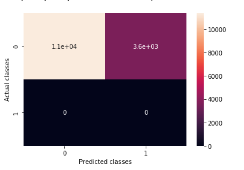
Plot Confusion Matrix

from sklearn.metrics import confusion_matrix




confusion_matrix(ytrain,pred_ytrain).ravel()


cfm = confusion_matrix(pred_ytrain,ytrain)
sns.heatmap(cfm, annot=True)
plt.xlabel('Predicted classes')
plt.ylabel('Actual classes')

Output:

Plot ROC

from sklearn.metrics import roc_curve, auc 

pred_test_log_prob=clf.predict_proba(xtrain)

fpr,tpr,_= roc_curve(ytrain,pred_test_log_prob[:,1])
roc_auc=auc(fpr,tpr)
print('area under the curve',roc_auc)
print('Accuracy',accuracy_score(ytrain,pred_ytrain))
plt.plot(fpr,tpr,label='ROC curve(area=%0.2f)' %roc_auc)
plt.xlabel('False Positive Rate')
plt.ylabel('True Positive Rate')
plt.title('Receiver operating charecteristic')
plt.legend(loc="lower right")
plt.show()

Output:

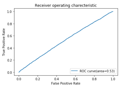
As we see our model is not performing well. Accuracy is just 0.76. Now we need to debug this. First anf foremost thing to check if there is any collinearity between the attributes with is disturbing the model

Collinearity Heat Map

corr=pdOneHotencoded[['Age','education-num','capital-gain','capital-loss','hours-per-week','salary']].corr(method='pearson')
print(corr)
#print(cor_df.corr(method='pearson').style.background_gradient(cmap='coolwarm'))
plt.figure(figsize=(10, 10))
plt.imshow(corr, cmap='coolwarm', interpolation='none', aspect='auto')
plt.colorbar()
plt.xticks(range(len(corr)), corr.columns, rotation='vertical')
plt.yticks(range(len(corr)), corr.columns);
plt.suptitle('NUmeric Data Correlations Heat Map', fontsize=15, fontweight='bold')
plt.show()

Output:

It seems there isn’t any correlation. There’s one more thing that needs to be checked Variation Inflation Factor.

Calculating VIF

from statsmodels.stats.outliers_influence import variance_inflation_factor
vif = pd.DataFrame()
Cont= pd.DataFrame()
cont=pdOneHotencoded[['Age','education-num','capital-loss','hours-per-week','capital-gain']]
vif["VIF Factor"] = [variance_inflation_factor(cont.values, i) for i in range(cont.shape[1])]
vif["features"] = cont.columns

print(vif)

Output:

VIF should be as low as possible. typically more than 10 is not acceptable.

Deleting Attributes with High VIF.

del pdOneHotencoded['Age']
del pdOneHotencoded['education-num']
del pdOneHotencoded['capital-loss']
del pdOneHotencoded['hours-per-week']
del pdOneHotencoded['capital-gain']

That’s it guys we have covered all the necessary steps required in basic data analysis of multidimensional data. Using these steps in the same sequence most types of data can be analyzed and the necessary inside can be developed.

Link to dataset and full code here