Weighted Least Squares Regression in Python

In this tutorial, we will learn another optimization strategy used in Machine Learning’s Linear Regression Model. It is the modified version of the OLS Regression. We will resume the discussion from where we left off in OLS. So, I recommend reading my post on OLS for a better understanding.

Weighted Least Squares (WLS)

If you know about the OLS, you know that we calculate the squared errors and try to minimize them. Now, consider a situation where all the parameters in the dataset don’t hold equal importance, or you would have felt that some parameters are more governing than others. In those cases, the variance of errors is not constant, and thus, the assumption on which OLS works gets violated.
Here comes the WLS, our rescuer. The modified version of OLS tackles the problem of non-constant variance of errors. It gives different weights to different variables according to their importance.

Mathematics behind WLS

Since we consider the weights of different variables according to their importance, the term used to minimize in the OLS equation changes. Instead of minimizing the squared errors, the weighted squared errors are minimized. This additional factor incorporated into the equation improves the fit as the data varies, resulting in a non-constant variance of errors. So, giving equal weights to all the independent variables will lead to biased and poor results.
The weights are generally calculated by taking the inverse of the variance of errors. If you get large weight variations, normalize it to have values with smaller variations. This will help our model to enhance the fitting process.

Let’s use the same Diabetes dataset that was used in the OLS.

Creating Residual Plot

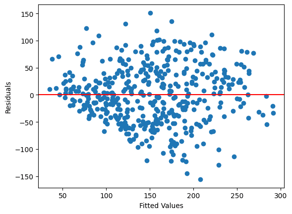
Let’s create the scatter plot between the residual values and fitted values of the OLS model. This will give the idea of whether our dataset has a non-constant variance of errors or not. The term for non-constant variance of errors is called heteroscedasticity. The cone-shaped plot indicates heteroscedasticity.

import matplotlib.pyplot as plt

X = df.drop('Target', axis=1)
y = df['Target']

X = sm.add_constant(X)

ols_model = sm.OLS(y, X)
ols_result = ols_model.fit()

plt.scatter(ols_result.fittedvalues, ols_result.resid)
plt.xlabel('Fitted Values')
plt.ylabel('Residuals')
plt.axhline(y = 0, color = 'r')
plt.show()

Calculating weights

As discussed above, the weights for the WLS model are generally calculated by taking the inverse of the variance of errors (residuals). Another way to calculate the weights is to know which variable or parameter is more important and then manually assign values.
To calculate the variance of residuals, we take the absolute values of residuals of current model as y and fittedvalues of the current model as X . Then we create our new OLS model and fit these new x and y. From the new model, we get the fittedvalues which are the standard deviation of the residuals. Therefore, to calculate the variance, take the square of it.

y_residual = [abs(residual) for residual in ols_result.resid]

X_residual = sm.add_constant(ols_result.fittedvalues)

model_residual = sm.OLS(y_residual, X_residual)
residual_result = model_residual.fit()

model_fv = residual_result.fittedvalues
variance = model_fv**2

weights = 1 / (variance)
print(weights)

0 0.000408 
1 0.000886 
2 0.000470 
3 0.000494 
4 0.000608  
... 
437 0.000434 
438 0.000715 
439 0.000634 
440 0.000398 
441 0.000982 
Length: 442, dtype: float64

Report of the Model

Let’s generate the report of the WLS model and compare it with the report of the OLS model. As you can see, the R2 value of OLS is 51.8, while that of WLS is 50.7. So, there is a decrease, and we can say that the WLS model explains less variance than the OLS model. You must be thinking that instead of increasing the value, it decreased. So, where did things go wrong?
The answer is that everything is correct. This happens when there is not a great violation of heteroscedasticity. This can also be seen from the plot. Take a look again, and now you will see that though the shape of a cone is present, the length of the cone is much smaller. We can conclude that homoscedasticity overpowers heteroscedasticity.
Another thing that can also be interpreted is whether the weights assigned by taking the inverse of the variance of residual hold good in this case or not. If we know which parameter has more importance and then assign weight accordingly, the model might be able to explain more variance. Think about it!

model = sm.WLS(y, X, weights = weights)
results = model.fit()


print(results.summary())