OLS Regression in Python – Ordinary Least Squares

This tutorial will explore the optimization strategy used often during the Linear Regression Model application in Machine Learning. Learn OLS regression in Python in depth.

Ordinary Least Squares (OLS)

Let’s first revise the working of the Linear Regression Model. The model tries to develop a linear relationship between independent variables, that is, (x), and dependent variables, that is, (y). The linear relationship means that any change in x will linearly change y. So, the model is trying to generate a straight line between y and x. Now, the straight line is governed by its slope and intercept. The best line will be the line that is closer to actual data points.
To find such a line, or you can say to govern the slope and intercepts, which are two crucial parameters, we use the optimization strategy called Ordinary Least Squares (OLS).

Mathematics behind OLS

The Linear Regression model aims to find parameters (slope and intercept) that minimize the difference between actual and predicted values. Since the error can be positive or negative, we can say the goal is to minimize the squared errors. Here comes the mathematics of OLS. It aims to minimize the sum of squared differences between actual and predicted values. You can also say that minimizing the squared errors.
If you are confused about the difference between linear regression and OLS, then to clear that, I would say read the aim of the linear regression model again. The major difference between them is how you minimize the error. OLS is just a method to minimize the error by minimizing the squared errors. There are various methods to minimize the error of the Linear Regression Model. OLS is just one of them.

Importing Libraries and Loading Dataset

Let’s code in Python and apply what we learned. So, first, import all the necessary libraries and load the dataset on which you would be applying the OLS approach. I am using the Diabetes dataset preloaded in the sklearn module.

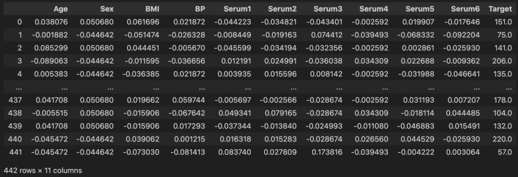
import pandas as pd
import numpy as np

import statsmodels.api as sm 
from sklearn import datasets
from sklearn.model_selection import train_test_split

diabetes = datasets.load_diabetes()

columns = ['Age', 'Sex', 'BMI', 'BP', 'Serum1', 'Serum2', 'Serum3', 'Serum4', 'Serum5', 'Serum6']
df = pd.DataFrame(data=np.c_[diabetes['data'], diabetes['target']], columns=columns + ['target'])
df

I am creating the DataFrame by concatenating the columns and providing column names for easier understanding.

Extracting the independent and dependent variables

You can see from the dataset that all the columns till Serum6 are independent variables, and the Target Column is our dependent variable. So, X will take all the values till the column name Serum6. Also, as you know, we must add a constant to the line equation. I am adding it using the statsmodel library.

X = df.drop('Target', axis=1)
X = sm.add_constant(X)
y = df['Target']

Report of the Model

We train the model and then print the report using model.summary()function. This detailed report contains the coefficients (slope in mathematical language and weights in Machine Learning language), F-statistic, R^{2  ,} which measures how well the model fits the data, and other statistical measures, including variance, covariance, and hypothesis testing.

model = sm.OLS(y, X).fit()
print(model.summary())