Optical Character recognition using Deep Learning (CNN)
 By Ripan Purkait
Our OCR (Optical Character Recognition) project aims to develop a robust and efficient system to detect characters and digits from an image. We are going to use Keras deep learning framework to implement our model. Keras is a TensorFlow-based API in Python.
Dataset Link:
https://www.kaggle.com/datasets/preatcher/standard-ocr-dataset
Link the Colab Notebook with Kaggle
!mkdir -p ~/.kaggle
!cp kaggle.json ~/.kaggle/
- Go to your Kaggle profile.
- Click on setting.
- Create an API key and download it.
- .Upload it in Colab.
Load the Dataset from Kaggle
! kaggle datasets download -d preatcher/standard-ocr-dataset
- Go to the dataset.
- Copy the API command and add an exclamatory(!) sign before it..
Unzip the File
import zipfile
zip_ref = zipfile.ZipFile('/content/standard-ocr-dataset.zip', 'r')
zip_ref.extractall('/content')
zip_ref.close()
zipfile.ZipFile('/content/standard-ocr-dataset.zip', 'r')– It creates a ZipFile object by specifying the path to the ZIP file and the mode is ‘r’, which stands for read-only.zip_ref. extractall ()– This line extracts all the contents of the ZIP file to the specified directory.zip_ref.close()–close()method is called on the ZipFile object to close the file after extraction, freeing up system resources.
Load the Libraries
import tensorflow as tf
from tensorflow import keras
from keras.models import Sequential
from keras.layers import Dense,Dropout,Flatten,Conv2D,MaxPooling2D
from PIL import Image
import matplotlib.pyplot as plt
from keras.utils import plot_model
import numpy as np
import matplotlib.pyplot as plt
import cv2
Display the Image from the Directory
#Specify the path to the image file
image_path = '/content/data/training_data/0/1008.png'

# Open the image using PIL
image = Image.open(image_path)

# Display the image using matplotlib
plt.imshow(image)
plt.axis('off')
plt.show()
Image.open()– It is used to open the image file by specified image path.plt.imshow(image)– It displays the image using theimshow()function from matplotlib.
Output
# Specify the path to the image file
image_path = '/content/data/training_data/1/10045.png'

# Open the image using PIL
image = Image.open(image_path)

# Display the image using matplotlib
plt.imshow(image)
plt.axis('off')
plt.show()
Output
# Specify the path to the image file
image_path = '/content/data/training_data/2/10046.png'

# Open the image using PIL
image = Image.open(image_path)

# Display the image using matplotlib
plt.imshow(image)
plt.axis('off')
plt.show()
Output
# Specify the path to the image file
image_path = '/content/data/training_data/3/10011.png'

# Open the image using PIL
image = Image.open(image_path)

# Display the image using matplotlib
plt.imshow(image)
plt.axis('off')
plt.show()
Output
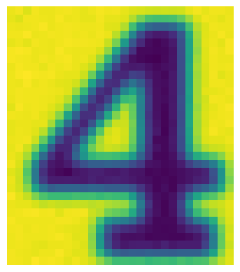
# Specify the path to the image file
image_path = '/content/data/training_data/4/10156.png'

# Open the image using PIL
image = Image.open(image_path)

# Display the image using matplotlib
plt.imshow(image)
plt.axis('off')
plt.show()
Output
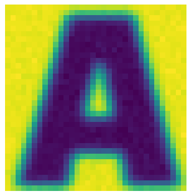
# Specify the path to the image file
image_path = '/content/data/training_data/A/10.png'

# Open the image using PIL
image = Image.open(image_path)

# Display the image using matplotlib
plt.imshow(image)
plt.axis('off')
plt.show()
Output
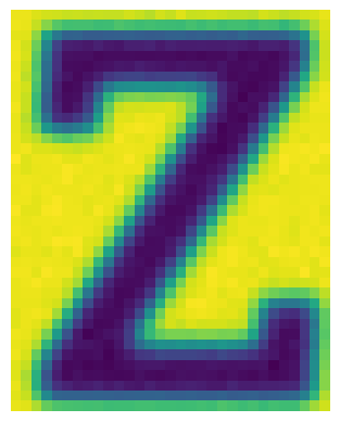
# Specify the path to the image file
image_path = '/content/data/training_data/Z/10007.png'

# Open the image using PIL
image = Image.open(image_path)

# Display the image using matplotlib
plt.imshow(image)
plt.axis('off')
plt.show()
Output
Loading and Preparing Image Datasets
train_df=keras.utils.image_dataset_from_directory(
     directory='/content/data/training_data',
     labels='inferred',
     color_mode = 'rgb',
     label_mode='categorical',
     batch_size=32,
     image_size=(224,224),
     shuffle=True
)
test_df=keras.utils.image_dataset_from_directory(
     directory='/content/data/testing_data',
     labels='inferred',
     color_mode = 'rgb',
     label_mode='categorical',
     batch_size=32,
     image_size=(224,224),
     shuffle=True
)directory– This line creates a training dataset using the images in the'/content/data/training_data'.labels– It means that the labels are automatically inferred from the directory structure.color_mode– It indicates that the images are in color.label_mode– It generates categorical labels.image_size– Set the desired image size.shuffle– shuffle the dataset randomly.
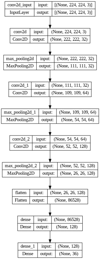
CNN Model
model = Sequential()
# convolutional layers
model.add(Conv2D(32, (3, 3), activation='relu', input_shape=(224,224, 3)))
model.add(MaxPooling2D((2, 2)))
model.add(Conv2D(64, (3, 3), activation='relu'))
model.add(MaxPooling2D((2, 2)))
model.add(Conv2D(128, (3, 3), activation='relu'))
model.add(MaxPooling2D((2, 2)))

# Flatten
model.add(Flatten())

# Dense layers
model.add(Dense(128, activation='relu'))
model.add(Dense(36, activation='softmax'))

# Compile the model
model.compile(optimizer='adam', loss='categorical_crossentropy', metrics=['accuracy'])
Model Architecture Visualization
plot_model(model, show_shapes=True, show_layer_names=True)
plot_model() – This function is used to visualize the model architecture.
Output
Model Training and Evaluation
history=model.fit(
    train_df,
    steps_per_epoch=len(train_df),
    epochs=50,
    validation_data=test_df,
    validation_steps=len(test_df)
)
model.evaluate(test_df)
train_df – This parameter is used to indicate that will be used to train the model. It should be a dataset object containing input images with their corresponding labels.
steps_per_epoch – It specifies the number of steps (batches) to be processed for each epoch during training.
epochs – This parameter will determine the no of times the entire training dataset will be iterated during training.
validation_data – It is used to specify the validation dataset, which is used to evaluate the model’s performance during training.
validation_steps – This parameter specifies the number of steps (batches) to be processed for validation during each epoch.
Output
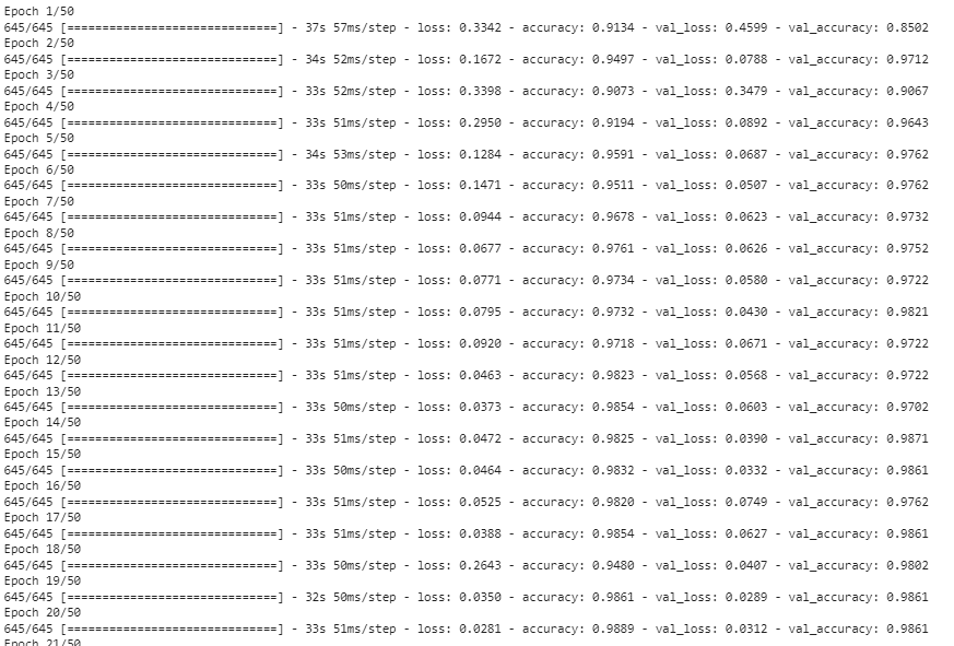
32/32 [==============================] - 1s 24ms/step - loss: 0.0244 - accuracy: 0.9881
[0.02437683567404747, 0.988095223903656]
Training and Validation Accuracy Visualization
plt.figure(figsize=(12,5))
plt.plot(history.history['accuracy'],color='red',label='train')
plt.plot(history.history['val_accuracy'],color='blue',label='validation')
plt.legend()
plt.show()
plt.figure(figsize=(12,5)) – This line creates a new figure of 12 inches in width and 5 inches in height. It set up the plotting area of the accuracy plot.
Output

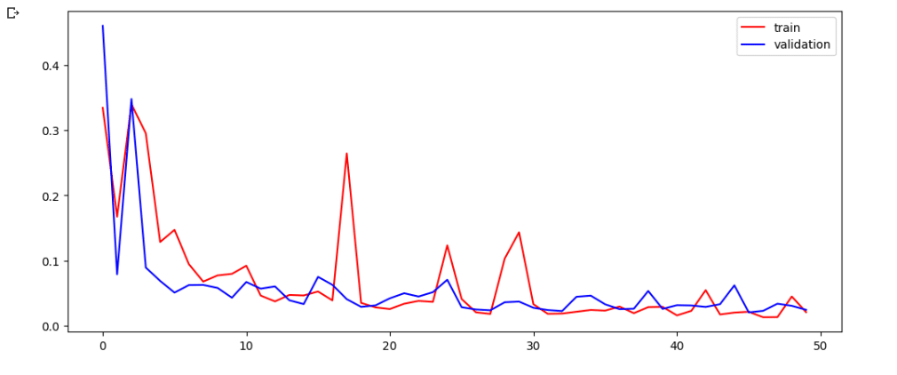
Training and Validation Loss Visualization
plt.figure(figsize=(12,5))
plt.plot(history.history['loss'],color='red',label='train')
plt.plot(history.history['val_loss'],color='blue',label='validation')
plt.legend()
plt.show()
Output
Save the Model
model.save('my_model.h5')model.save() – This method is an object of the model that allows us to save our model in HDF5(.h5) format.
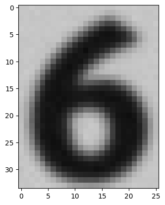
Let’s test our model with some random image
test_img = cv2.imread('/content/data2/training_data/6/44482.png')
plt.imshow(test_img)
test_img.shape
test_img = cv2.resize(test_img,(224,224))
test_input = test_img.reshape((1,224,224,3))
model.predict(test_input)
cv2.imread() – This function reads an image file using the openCV imread() function.
cv2.resize() – This function resizes the image to a specified size using the openCV resize() function.
test_image.reshape() – This line reshapes the test_img image into a 4-dimensional array with shapes (1, 224, 224, 3). It adds an extra dimension to represent the batch size of 1, as expected by the model for prediction.
Output
1/1 [==============================] - 0s 19ms/step
array([[2.9703050e-12, 0.0000000e+00, 9.6275628e-36, 2.6602739e-20,
        1.3241535e-22, 1.0799878e-12, 1.0000000e+00, 0.0000000e+00,
        2.5963045e-17, 1.1112179e-24, 1.8801211e-15, 8.2622201e-17,
        4.5579626e-16, 2.7424159e-29, 5.7890647e-21, 5.8862996e-25,
        1.0082446e-12, 8.9091432e-27, 5.1499902e-25, 1.3380033e-25,
        2.6840049e-27, 1.5669024e-22, 5.6188350e-29, 1.5992485e-34,
        9.9730228e-17, 3.8556169e-34, 4.0268902e-29, 6.1393704e-26,
        5.1515190e-19, 2.0781772e-30, 1.1479811e-29, 4.9926123e-31,
        7.3255638e-32, 3.2171518e-35, 1.3497997e-32, 2.0042042e-31]],
      dtype=float32)
predictions = np.array([[2.9703050e-12, 0.0000000e+00, 9.6275628e-36, 2.6602739e-20,
1.3241535e-22, 1.0799878e-12, 1.0000000e+00, 0.0000000e+00,
2.5963045e-17, 1.1112179e-24, 1.8801211e-15, 8.2622201e-17,
4.5579626e-16, 2.7424159e-29, 5.7890647e-21, 5.8862996e-25,
1.0082446e-12, 8.9091432e-27, 5.1499902e-25, 1.3380033e-25,
2.6840049e-27, 1.5669024e-22, 5.6188350e-29, 1.5992485e-34,
9.9730228e-17, 3.8556169e-34, 4.0268902e-29, 6.1393704e-26,
5.1515190e-19, 2.0781772e-30, 1.1479811e-29, 4.9926123e-31,
7.3255638e-32, 3.2171518e-35, 1.3497997e-32, 2.0042042e-31]])
# Find the index of the maximum value
index_of_max = np.argmax(predictions)
# Get the maximum value
max_value = predictions.flatten()[index_of_max]
print('Maximum value:', max_value)
Output
Maximum value: 1.0
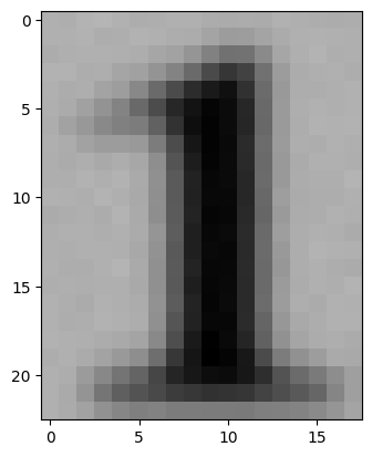
test_img = cv2.imread('/content/data2/testing_data/1/44245.png')
plt.imshow(test_img)
test_img = cv2.resize(test_img,(224,224))
test_input = test_img.reshape((1,224,224,3))
model.predict(test_input)
Output
test_img = cv2.imread('/content/data2/testing_data/Z/43595.png')
plt.imshow(test_img)
test_img = cv2.resize(test_img,(224,224))
test_input = test_img.reshape((1,224,224,3))
model.predict(test_input)
Output
Leave a Reply