Anomaly Detection Using TensorFlow and Autoencoders
 By Satyam Prashant
Due to technological growth, there has been a steep rise in fraud and illegal activities, particularly in the financial sector. There is a need for a highly effective algorithm that monitors data flow behaviors, identifies patterns, and has the capability to anticipate irregularities or instances of fraud. This efficient algorithm is built using autoencoders. This tutorial will dive deep into the utilization of autoencoders in anomaly detection using TensorFlow and other Python libraries.
Introduction To Autoencoders
An autoencoder is a kind of neural network architecture that effectively reduces input data to its most basic components through compression (encoding) and then uses this compressed representation to reconstruct (decode) the original input.
A few key concepts of autoencoders used in anomaly detection are:
- There are 3 layers in autoencoders. The layers are the decoder layer, the encoder layer, and the bottleneck layer. The encoder begins by condensing the input data into a smaller encoded data set, therefore encoding the intricate feature patterns seen in the data. An important element is the bottleneck layer, which serves as a feature space where anomalies are anticipated to be less well-represented and displays the input data in its compressed form.
- Autoencoders are generally trained on a large dataset with normal instances. The model generated is then capable of encoding and reconstructing the normal data accurately.
- After training the model, it is capable of detecting anomalies. It does so using a concept called reconstruction error, i.e., how much the reconstructed data differs from the original. If the difference is significant, we categorize it into an anomaly.
- We will be using tanh and ReLu activation functions because they provide better performance for multi-layer neural networks and also because ReLu can solve the solve the vanishing gradient problem that the sigmoid function suffers from.
Code Implementation in Python
Importing The Necessary Python Libraries
import numpy as np
import pandas as pd
from sklearn.model_selection import train_test_split
from sklearn.preprocessing import StandardScaler, MinMaxScaler
from sklearn.metrics import accuracy_score
import tensorflow as tf
from tensorflow.keras import layers, models
import matplotlib.pyplot as plt
Dataset Preprocessing and loading
Dataset download link: Download the dataset
This dataset consists of credit-card transactions. We will remove the “Time” column and use one-hot encoding for the target column. The dataset will then be divided into training and testing sets in an 80:20 ratio.
# Loading the dataset
df_credit = pd.read_csv('creditcard.csv')
# Dropping the 'Time' column
df_credit = df_credit.drop(['Time'], axis=1)

# Standardizing and scaling the features to the range of (-1,1)
scaler_data = StandardScaler()
df_credit['Amount'] = scaler_data.fit_transform(df_credit['Amount'].values.reshape(-1, 1))

# Convert Class column into a string
df_credit['Class'] = df_credit['Class'].astype(str)

# one-hot encoding for the 'Class'
df_credit = pd.get_dummies(df_credit, columns=['Class'], prefix=['Class'])

# Splitting the dataset into training and testing
train, test = train_test_split(df_credit, test_size=0.20, random_state=42)

# Extract features and labels
x_train = train.drop(['Class_0.0', 'Class_1.0'], axis=1).values
y_train = train[['Class_0.0', 'Class_1.0']].values

x_test = test.drop(['Class_0.0', 'Class_1.0'], axis=1).values
y_test = test[['Class_0.0', 'Class_1.0']].values
Handling the missing values
the missing values present in the test and train datasets after splitting is replaced by the mean values of the features using impute function of sklearn library.
#impute the missing values (nan) with the mean
from sklearn.impute import SimpleImputer
imputer = SimpleImputer(missing_values=np.nan, strategy='mean')
x_test = imputer.fit_transform(x_test)
Model Training
We will train the model for 10 epochs. For better results, it is also recommended to go up to 25 epochs. We will build our model layer by layer: encoder, bottleneck, and decoder layers. Since our data is scaled to the range (-1,1), we will use the ‘tanh’ activation function. The loss function used to evaluate the model is Mean Squared error (MSE).
# Converting train and test data to 'int' datatype
x_train = x_train.astype(int)
x_test = x_test.astype(int)

# building autoencoder function
def Auto_Encoder(input_shape):
    """

    Args:
      input_shape:

    Returns:

    """
    model = models.Sequential()
    # Encoding layer
    model.add(layers.InputLayer(input_shape=input_shape))
    model.add(layers.Dense(64, activation='relu'))
    model.add(layers.Dense(32, activation='relu'))

    # bottleneck layer
    model.add(layers.Dense(16, activation='relu'))
    # Decoding layer
    model.add(layers.Dense(32, activation='relu'))
    model.add(layers.Dense(64, activation='relu'))
    model.add(layers.Dense(input_shape, activation='tanh'))
    return model

input_shape = x_train.shape[1]
autoencoder = Auto_Encoder(input_shape)

# Compile the Model
autoencoder.compile(optimizer='rmsprop', loss='mse', metrics=['accuracy'])

# Train the Autoencoder
history = autoencoder.fit(x_train, x_train, epochs=10, batch_size=64, shuffle=False, validation_data=(x_test, x_test))
Output :
Epoch 1/10 2403/2403 [==============================] - 7s 2ms/step - loss: 0.3972 - accuracy: 0.7286 - val_loss: 0.3545 - val_accuracy: 0.7452
Epoch 2/10 2403/2403 [==============================] - 6s 2ms/step - loss: 0.3537 - accuracy: 0.7494 - val_loss: 0.3430 - val_accuracy: 0.7672
Epoch 3/10 2403/2403 [==============================] - 7s 3ms/step - loss: 0.3476 - accuracy: 0.7669 - val_loss: 0.3385 - val_accuracy: 0.7930
Epoch 4/10 2403/2403 [==============================] - 5s 2ms/step - loss: 0.3447 - accuracy: 0.7721 - val_loss: 0.3352 - val_accuracy: 0.8136
Epoch 5/10 2403/2403 [==============================] - 7s 3ms/step - loss: 0.3426 - accuracy: 0.7808 - val_loss: 0.3322 - val_accuracy: 0.7741
Epoch 6/10 2403/2403 [==============================] - 5s 2ms/step - loss: 0.3412 - accuracy: 0.7874 - val_loss: 0.3302 - val_accuracy: 0.7848
Epoch 7/10 2403/2403 [==============================] - 7s 3ms/step - loss: 0.3402 - accuracy: 0.7911 - val_loss: 0.3295 - val_accuracy: 0.7884
Epoch 8/10 2403/2403 [==============================] - 6s 2ms/step - loss: 0.3394 - accuracy: 0.7925 - val_loss: 0.3299 - val_accuracy: 0.7906
Epoch 9/10 2403/2403 [==============================] - 6s 2ms/step - loss: 0.3387 - accuracy: 0.7939 - val_loss: 0.3286 - val_accuracy: 0.7900
Epoch 10/10 2403/2403 [==============================] - 6s 3ms/step - loss: 0.3381 - accuracy: 0.7952 - val_loss: 0.3285 - val_accuracy: 0.7884
Plotting Training and Validation Results
We will try to see how loss and accuracy change with the number of epochs for both the training set and the validation set of our dataset.
# plotting loss and accuracy against no. of epochs
plt.figure(figsize=(10, 3))

# for training metrics
plt.subplot(1, 2, 1)
plt.plot(history.history['loss'], label='Training Loss', color = 'blue')
plt.plot(history.history['accuracy'], label='Training Accuracy', color = 'green')
plt.title('Training')
plt.xlabel('Epochs')
plt.ylabel('Loss and Accuracy')
plt.legend()

# for validation metrics
plt.subplot(1, 2, 2)
plt.plot(history.history['val_loss'], label='Validation Loss', color = 'red')
plt.plot(history.history['val_accuracy'], label='Validation Accuracy', color = 'orange')
plt.title('Validation')
plt.xlabel('Epochs')
plt.ylabel('Loss and Accuracy')
plt.legend()

plt.tight_layout()
plt.show()
Output :
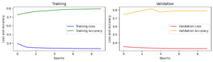
As we can see, with the increase in the number of epochs, the loss decreases and accuracy increases. Therefore, we can conclude that the increase in the number of training epochs will increase the model’s performance.
Evaluating accuracy of the Model
# Evaluating the function
predicted_values = autoencoder.predict(x_test)
mse = np.mean(np.power(x_test - predicted_values, 2), axis=1)

# Setting threshold for anomalies
threshold = 0.5

# Classifying anomaly detection condition
anomalies = mse > threshold

# Evaluating the detection model
y_true = np.argmax(y_test, axis=1)
y_pred = anomalies.astype(int)

print(f'Test Accuracy: {accuracy_score(y_true, y_pred):.4f}')
Output :
1202/1202 [==============================] - 2s 1ms/step
Test Accuracy: 0.9427
For better performance accuracy we can use hyper parameter tuning and feature engineering. For more information on how to improve model accuracy, check it.
Plotting the detected anomalies
# plot for detected anomalies
plt.figure(figsize=(8, 3))
plt.scatter(range(len(mse)), mse, c=anomalies, cmap='Accent', s=5)
plt.title('Anomaly detection')
plt.xlabel('Observations')
plt.ylabel('MSE')
plt.tight_layout()
plt.show()
Output :
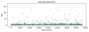
We can clearly observe from this scatter-plot, the anomalies are the data points with greater MSE than threshold. The points near to the base line are with MSE 0. Therefore, points with higher MSE are detected as anomalies.
Leave a Reply