Calculate F1 Score using sklearn in Python

In this tutorial, I will guide you through what the F1 score is, what is the need to use it, and how to calculate the F1 score.

F1 Score

Before you study what the F1 score means, let us explore the situations or instances why the F1 Score is needed, as we already have accuracy for evaluating the model. Let’s remember the formula of accuracy :
Accuracy = Number of correct predictions / Total number of predictions

Do you think it is enough?
Let us understand it with an example. Consider the scenario where 1000 people go to detect COVID using method 1. They also undergo RT-PCR test for the same. Assuming RT-PCR gives the result with 100% accuracy, this is what is observed:

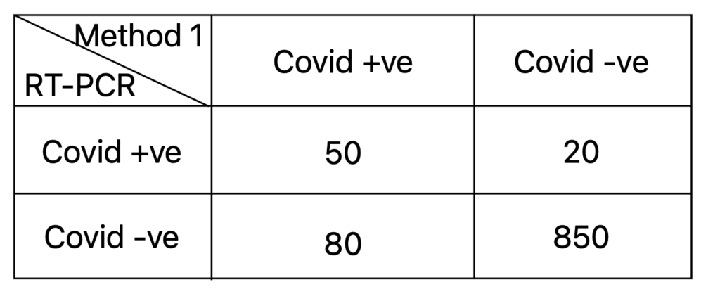
Let’s calculate the accuracy for method 1 here, which comes out to be 90% ((850+50)/1000).

Consider another scenario where 1000 people go to a magician to detect Covid. They also undergo RT-PCR test for the same. Assuming RT-PCR gives the result with 100% accuracy, this is what is observed:

Calculating the accuracy for magician here, which comes out to be 93% (930/1000). So, can you conclude that the magician is better than method 1?

Thus, the F1 score comes to our rescue. The F1 Score measures the model’s accuracy by taking the harmonic mean of Recall and Precision scores.

Precision: It measures how many positive predictions made by the model are correct.
Recall: It measures how many positive class samples in the dataset are correctly identified by the model.

A higher precision score means a strict classifier will doubt the true positive samples, reducing the recall score. In contrast, a higher recall score means a lenient classifier will pass those samples, which resembles a positive class, reducing the precision score. Thus, we want to maximize the precision and recall scores, so if we maximize the F1 score, precision and recall scores will automatically be maximized.

Precision (P) = (TP)/(TP + FP)
Recall (R) = (TP)/(TP + FN)
F1 Score = (2PR)/(P + R)

Step 1: Importing Libraries

Import all the necessary libraries.

from sklearn.model_selection import train_test_split
from sklearn.linear_model import LogisticRegression
from sklearn.metrics import f1_score,accuracy_score, classification_report, confusion_matrix
from sklearn.datasets import load_iris

import seaborn as sns
import matplotlib.pyplot as plt

Step 2: Loading the Dataset

I will be using the iris dataset from the sklearn datasets.

iris = load_iris()
X, y = iris.data, iris.target

Step 3: Train the model and make Predictions

Let’s go with the Logistic Regression model. First, split your dataset into a training set and a test set. I am splitting in the ratio of 70:30, respectively. I am also taking the random seed, so you will get the same results every time you run it.

X_train, X_test, y_train, y_test = train_test_split(X, y, test_size=0.3, random_state=2023)

model = LogisticRegression()
model.fit(X_train, y_train)

y_pred = model.predict(X_test)

Step 4: Calculating the F1 score and accuracy

Let’s see the F1 score and accuracy of the model.

f1 = f1_score(y_test, y_pred, average='weighted')
print(f'F1 Score: {f1:.4f}')

accuracy = accuracy_score(y_test, y_pred)
print(f'Accuracy: {accuracy:.4f}')

You will see the following output:

F1 Score: 0.9776 
Accuracy: 0.9778

The parameter average='weighted' considers how you want to calculate the F1 score. The default value is binary, but our dataset is multi-class so we are passing weighted as argument.

More Information

Let’s also print the classification report of the model, which will contain the recall and precision scores of the class.

print("Classification Report:\n", classification_report(y_test, y_pred))

Output:

Using Heatmap from Seaborn, let’s also visualize the matrix to understand the True positives, negatives, False positives, and False negatives.

cm = confusion_matrix(y_test, y_pred)

plt.figure(figsize=(6, 4))
sns.heatmap(cm, annot=True, fmt='d', cmap='Blues', xticklabels=iris.target_names, yticklabels=iris.target_names)
plt.xlabel('Predicted')
plt.ylabel('True')
plt.title('Confusion Matrix')
plt.show()

Output: